🌲 Day 4: Statistics Enchanted Forest#
Join Oda the Data Otter as she explores the enchanted Statistics Forest, where magical creatures reveal the secrets of mean, median, sampling, and bootstrap magic through epic adventures and mystical challenges!
🎯 Learning Objectives#
📊 Become human data points and discover mean, median, and mode through the “Human Histogram” adventure
🔍 Master distribution detective skills to identify symmetrical, left-skewed, and right-skewed data patterns
🎲 Understand the difference between populations and samples through magical creature studies
📏 Discover how sample size affects the reliability of our statistical conclusions
🎃 Experience sampling variability through the Halloween candy discovery adventure
🐑 Learn bootstrapping magic by rescuing sheep from dragon fire
🎯 Build confidence intervals to make educated guesses about unknown populations

✨ Extra Challenge (Optional)
Ready for something more challenging? Try these extra challenging scripts in Posit Cloud!:
Work through the extra challenging worksheet
activities/day04_extra_challenge.Rmd.If you get stuck, reach out to your instructor for help!
📥 How to Download Your Folder/Files from Posit Cloud#
Follow these quick steps to save your work to your computer:
In Posit Cloud, open the Files pane (bottom-right).
Click the checkbox next to the folder or files you want (for example,
day04/or a single.Rmd).Click More (with blue gear icon) → Export.
A
.zipfile will download with your selected items.
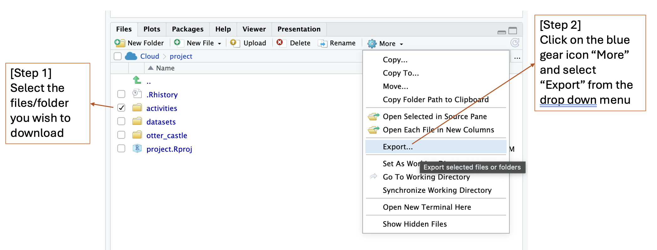
💡 Pro tip: If you don’t select anything, Export will download the current folder you’re viewing.
1. 🎈 Ice Breaker Activity: Human Histogram & Statistics Discovery#
Duration: 30 minutes
🎉 Today, YOU become the data points! We’ll use our own heights and birthdays to discover the magic of mean, median, and mode.
1.1 Height Histogram & Mean Discovery#
Duration: 20 minutes
🧙♀️ Human Lineup: Line up by height from shortest to tallest
🔍 In-Person Investigation:
Find the shortest wizard (minimum)
Find the tallest wizard (maximum)
Find the middle wizard (median) - count from both ends!
📝 Data Collection: Enter your wizard name and height into our magical data form: https://forms.gle/TG2dgNwknN6KGTcE6
📏 What if I don’t know my height?:
Try to give a guess about your height using reference objects or people around you.
For example, a regular paper is 21 cm in width and 30 cm in height.
Your instructor Sky is 175 cm tall.
🧮 Calculate Our Class Mean Height: We’ll add up everyone’s heights and divide by the number of wizards in our class
💻 R Magic Verification: Watch as we put your data into R and compare our human results with computer calculations!
🤔 Why Do We Care About Mean?
The mean tells us what a “typical” wizard in our class looks like!
Other examples of using Mean:
🌡️ Weather Wizard: Weather apps use mean temperature to tell you if it’s a hot or cold month
🏀 Sports Star: Basketball players track their mean points per game to see how good they are
🍕 Pizza Party Planning: If you know the mean number of pizza slices each friend eats, you can order the right amount!
1.2 Birthday Block Building & Mode/Median Discovery#
Duration: 15 minutes
📅 Which Month Is Your Birthday?:
💻 R Data Collection: We’ll enter each wizard’s birth month into our R list
📊 Visual Discovery: Watch our classroom histogram grow in real-time!
🔍 Statistical Magic:
Find the mode (tallest stack = most popular month)
Calculate the mean month using R
🤔 Pattern Spotting: Which months are popular? Any empty months?
💡 Pro Tips: Different types of data need different measures!
Mean = Add everyone’s height up and divide by total number of students in the class
Median = Middle detective in a lineup of counts
Mode = Most popular birthday month in the room
🤔 Why Do We Care About Median?
The median shows us the “middle” value that splits our data in half!
Other examples of using Median:
🏠 House Prices: When some houses cost millions and others cost thousands, median gives a better “typical” price than mean
🍎 Test Scores: Median helps teachers see how the “middle” student performed, not affected by super high or low scores. This helps teachers to see how well the class in general understands a new concept.
🤔 Why Do We Care About Mode?
The mode tells us what happens most often - the most popular choice!
Other examples of using Mode:
👕 T-Shirt Sizes: Stores need to know which size sells most (mode) to stock the right amounts
🍦 Ice Cream Flavors: Ice cream shops track which flavor is ordered most often to plan their inventory

2. Distribution Detective Mission 🔍#
Duration: 35 minutes
2.1 The Shape of Data Magic#
Duration: 5 minutes
💡 What are Data Distributions? Just like how people can be tall, short, or in-between, data comes in different shapes! Some data is perfectly balanced (symmetrical), some leans to one side (skewed), and some has unusual outliers that surprise us.
Today’s Mission: Investigate three magical creature types with completely different distributions!
Spell 1: Distribution Detective Investigation#
Duration: 30 minutes
🎈 Activity: The Three Magical Distribution Mysteries#
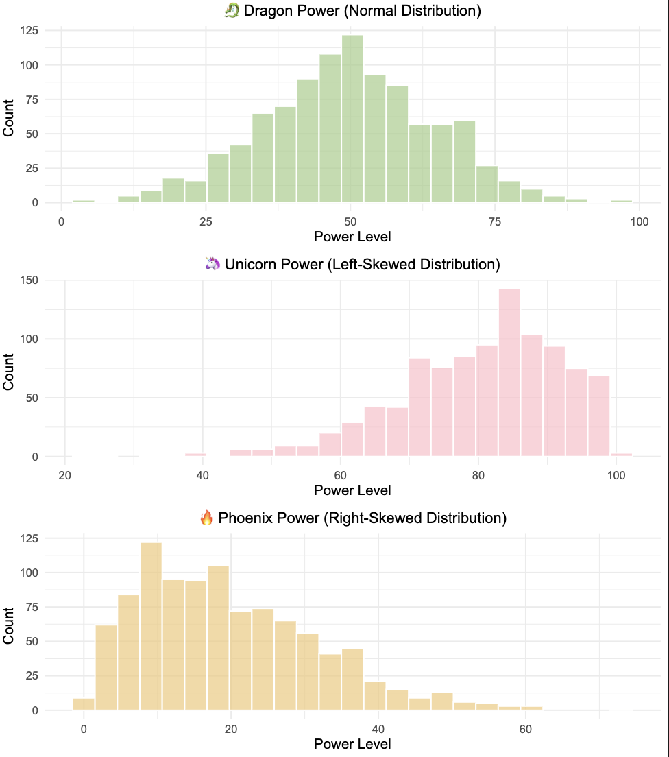
🐉 Mystery 1: Dragon Power (Symmetrical Distribution)
Most dragons have medium power
Few dragons are very weak or very strong
Mean and median are best friends (very close together)!
🦄 Mystery 2: Unicorn Magic (Left-Skewed Distribution)
Most unicorns have high magic
A few unicorns have very low magic (creates a “tail” on the left)
Mean gets “pulled down” by the low values
🔥 Mystery 3: Phoenix Energy (Right-Skewed Distribution)
Most phoenixes have low energy
A few phoenixes have extremely high energy (creates a “tail” on the right)
Mean gets “pulled up” by the high values
📁 Find this spell in Posit Cloud: Look for the file day04_spell01_distribution_detective.Rmd in your project files!
🔍 Detective Challenge Questions:
Which creature type has mean and median closest together? Why?
Which creature type shows the biggest difference between mean and median?
When data is skewed, which is better to use: mean or median?

💡 Detective Rules:
Symmetrical data: Mean ≈ Median (use either one!)
Left-skewed distributions: Mean < Median (mean gets pulled down because of outliers with small values sitting on the left side)
Right-skewed distributions: Mean > Median (mean gets pulled up because of outliers with large values sitting on the right side)
When data is skewed, median is often a better measure of “typical” value
Outliers: Can pull the mean away from where most data sits
3. 🎲 The Great Sampling Adventure#
Duration: 65 minutes
3.1 Game 1: The Enchanted Halloween Neighborhood Mystery 🎃#
Duration: 25 minutes
3.1.1 🎈 Activity: Statistical Wizards Save Halloween#
📖 The Story:
The Mgaic Council of Halloween has received reports that the Shadow Monster has been cursing neighborhoods, turning precious candies into worthless shadow stones! As young Statistical Wizards, your mission is to determine if the Enchanted Forest Neighborhood is safe for trick-or-treating.
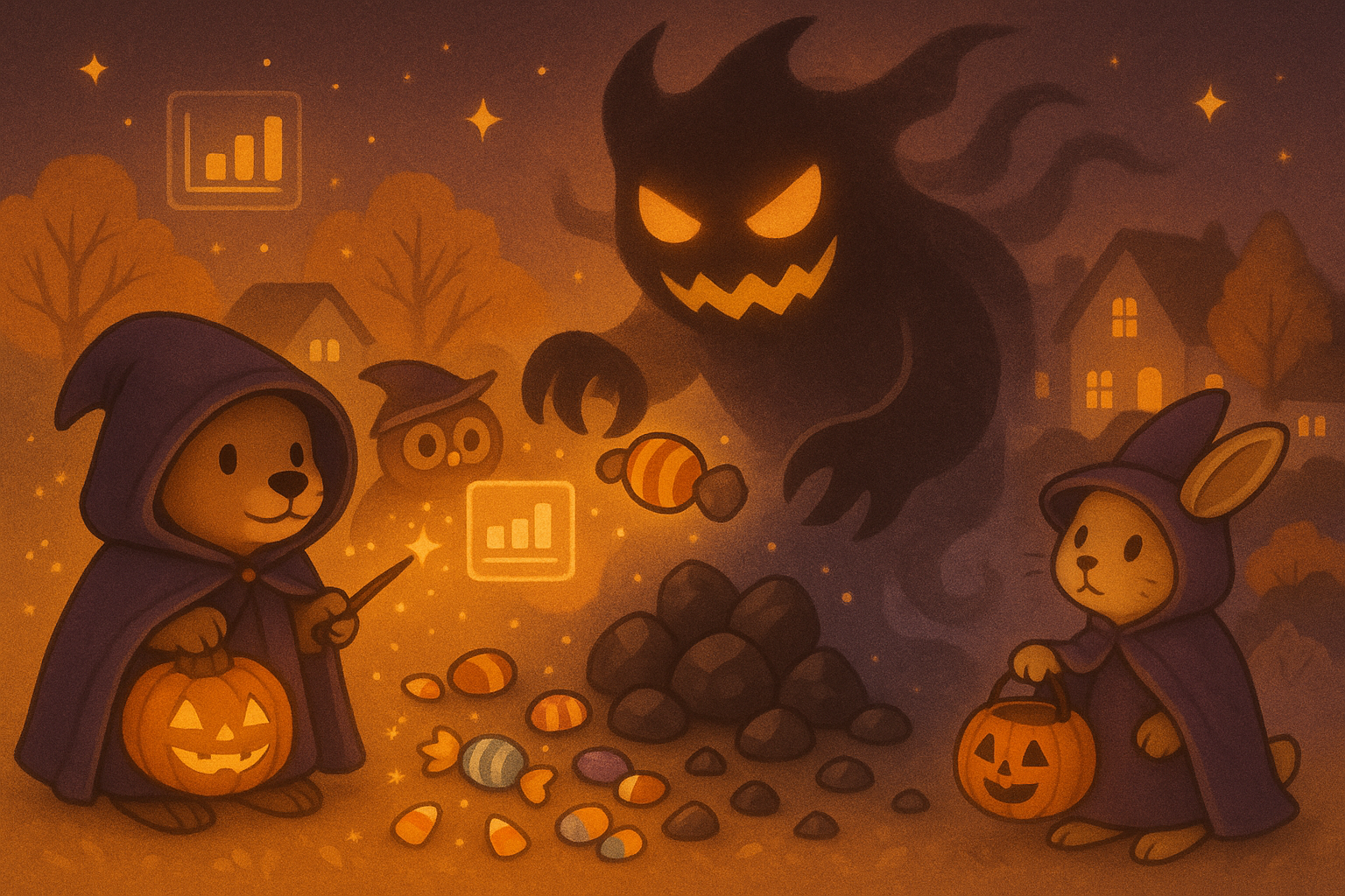
⚡ The Challenge:
The neighborhood has a magical protection spell - if it contains 60% or more real candies (not shadow stones), it’s safe to visit. But beware! You only have 3 minutes of magical sight to examine your sample before the spell fades.
🧙♀️ You will get:
The Mgaic Council Has Prepared “Time Crystal Bag” for everyone. You will each get one “Time Crystal Bag” containing 10 items
⚡ The Magic Rules:
Incantation Phase: You will chant “Statistical powers, reveal the truth!” before opening your bags
Counting Phase: 3 minutes for magical sighting to count candies vs. shadow stones
Decision Phase: Each wizard declares if they think the neighborhood is “SAFE” or “CURSED”
Data Crystal Phase: Enter candy count, and your decision into the magical Google Form: https://forms.gle/pVVK2zBVovA1637Z9

💡 The Magic Discovery: Different samples give different results! This is called sampling variability - and it’s totally normal!
3.1.2 🎈 Activity: Statistical Wizards Save Halloween - Round 2!!#
Duration: 25 minutes
🎉 Good News! The magical council has prepared more “Time Crystal Bag” for us!
🪄 You will get:
Everyone gets 1 more “Time Crystal Bag”
⚡ The Magic Rules:
Incantation Phase: you will chant “Statistical powers, reveal the truth!” before opening their bags
Counting Phase: 5 minutes to count candies vs. shadow stones (how many candies do you have total among the 20 items you got from 2 bags!)
Decision Phase: Each wizard declares if they think the neighborhood is “SAFE” or “CURSED”
Data Crystal Phase: Enter candy count, and your decision into the magical Google Form: https://forms.gle/dwMLreYBN4CHmWwh8
🏆 Rewards & Competition:
Prediction Points: Kids who make the right prediction earn rewards!
3.1.3 💡 Pro Tips: Understanding Sampling Magic#
Duration: 5 minutes
🎯 What is a Sampling Distribution? Remember our candy bag game? Imagine if 100 different kids each got their own “Time Crystal Bag” with 10 items from the same magical neighborhood. Each kid counts their candies and gets a different result - maybe 6 candies, 8 candies, 7 candies, etc. If we collected ALL 100 results and made a graph showing how many kids got 6 candies, how many got 7, etc., that graph is called a sampling distribution! It shows us the pattern of what happens when lots of samples are taken from the same population.
📊 What is Spread (Variability)? Spread tells us how “spread out” or scattered our data points are:
Small spread: All your data points are close together (like 28%, 30%, 32% candies)
Large spread: Your data points are far apart (like 15%, 30%, 45% candies)
Magic Rule: Larger samples = smaller spread = more reliable results!
🧮 What Does the Mean of the Sampling Distribution Tell Us? Here’s the coolest part about our candy bag game! Let’s say the magical neighborhood actually has 20% candies. If 100 kids each count their bags, some might get 1 candies, some 2, some 3, etc. But here’s the magic: if you add up ALL their candy counts and find the average, you’ll get very close to 2 candies (which equals 20%)! Even though each kid got different results, when we combine everyone’s results, we get closer to the truth about the neighborhood!
🔍 Real-Life Example: If the true percentage of dragons in the forest is 30%, and you take 100 different samples:
Some samples might give you 25% dragons
Some might give you 35% dragons
But the AVERAGE of all 100 sample percentages will be very close to 30%!

3.2 Understanding Populations vs Samples#
Duration: 5 minutes
💡 The Big Picture: Imagine you want to know what percentage of creatures in the entire Enchanted Forest are dragons, but you can’t count all million creatures! So you explore small areas and use those to make educated guesses.

🌲 Population = All creatures in the entire Enchanted Forest (everything we want to know about)
🔍 Sample = The creatures we find in one small area (the small group we actually study)
🎯 Parameter = The true characteristic of the entire population (like “exactly 30% of all forest creatures are dragons”)
📊 Statistic = Something we calculate from our sample (like “25% of creatures in our sample are dragons”)
🎯 Inference = Using our sample to make conclusions about the whole population, knowing how uncertain we are
3.2.1 🎈 Activity: The Magical Creature Population Study#
Duration: 20 minutes
🐉 The Setup: In the Enchanted Forest, we have a population of 1000 magical creatures where exactly 30% are dragons. Let’s see what happens when we take different sized samples!
📁 Find this spell in Posit Cloud: Look for the file day04_spell02_sampling_adventure.Rmd in your project files!
🔬 The Three Great Experiments:
Small Samples (Size 20): Take 300 samples of 20 creatures each
Medium Samples (Size 40): Take 300 samples of 40 creatures each
Large Samples (Size 200): Take 300 samples of 200 creatures each
🎯 Key Discoveries:
All sample sizes give averages close to the truth (30% dragons)
Larger samples are more reliable
Sampling distributions form beautiful bell shapes!
The spread decreases as sample size increases
💡 The Magic Moment: When we increase sample size, we make our estimates much more reliable!
4. 🐑 The Great Dragon Fire Sheep Rescue#
Duration: 65 minutes
4.1 Understanding Bootstrap Magic & Confidence Prophecies#
Duration: 5 minutes
💡 The Big Picture: Imagine you’re a shepherd trying to count sheep in a thick fog! You can only see a small group at a time, but you need to know about the entire flock. Bootstrap magic lets you use your small sample to imagine what hundreds of other samples might look like!
🐑 Bootstrap Magic = Using your small sheep sample to create hundreds of “pretend samples” with replacement
🎯 Confidence Prophecy = Your estimate range: “I’m 90% confident the true percentage is between X% and Y%”
🔮 The Magic Hat Rule = Always put the sheep back! (sampling WITH replacement)
🎯 Inference Goal = Use your small flock sample to make educated guesses about the entire meadow
4.1.1 What is Bootstrapping?#
Duration: 2 minutes
The word bootstrapping comes from the saying “pulling yourself up by your bootstraps,” which means doing something hard without outside help. Here, the hard job is to estimate a population value and explain how precise our estimate is—using only one sample of data.
This approach only works well if the original sample represents the population. We treat that sample as a stand‑in for the whole population—that’s the key idea of bootstrapping. This connects back to why good sampling methods matter, just like we discussed earlier.
4.1.2 What are the basic bootstrapping steps?#
Draw a bootstrap sample: randomly sample with replacement from the original data until you have the same size \(n\).
Compute the statistic (point estimate) on that bootstrap sample.
Repeat steps (1) and (2) \(b\) times to build the bootstrap distribution—the collection of those point estimates.
Use that distribution to find a plausible range for the parameter (an empirical confidence interval).
4.2 Game 1: The Great Dragon Fire Sheep Rescue 🐑🔥#
Duration: 30 minutes
4.2.1 🎈 Activity: Bootstrap Magic & Confidence Prophecies#
📖 The Story:
URGENT QUEST ALERT! The ancient Dragon of Mount Statistics has accidentally breathed fire across the Enchanted Meadows, where Farmer Luna (white sheep) and Farmer Obsidian (black sheep) graze their magical flocks. The fire didn’t harm the sheep, but created a massive cloud of magical smoke that mixed all the flocks together!
The two farmers are worried and need to know how many of their sheep are mixed together in the smoky field. But here’s the problem: the smoke is so thick that shepherds can only see a small group of sheep at a time, and all the water was used to put out the fire, so they can’t wash the sheep to see their true colors clearly!
⚡ The Challenge:
As Junior Statistical Shepherds, you must use the ancient art of Bootstrap Magic to estimate what percentage of the total flock is black sheep, and create a Confidence Prophecy (confidence interval) for your estimate.
🪄 You will get:
Everyone gets to take random samples from the smoke sample bag (easier to count if you only take 10)
⚡ The Rescue Rules:
Initial Vision Phase: Count black vs. white sheep in your original sample
Percentage of Black Sheep: Calculate and write down what’s the percentage of black sheep in your sample
Bootstrap Prophecy Phase: Use magic hat sampling to create > 3 bootstrap samples
Remember to write down the percentage of black sheep in each bootstrapped sample!
Confidence Prophecy Phase: Calculate your 90% confidence interval for black sheep percentage using the code below (if you have trouble calculating this, raise your hand and get help from your instructor and mentors!):
# enter the percentage of black sheep in each of your bootstrapped sample below:
# for example:
black_percentage <- c(0.5, 0.6, 0.7)

# calculate 90% confidence interval
confidence_interval <- quantile(black_percentage,
                               probs = c(0.05, 0.95))
Royal Registry Phase: Write down your confidence prophecy on a piece of paper
🎯 Bootstrapping Example – Sheep Edition You can only see 20 sheep through the smoke, but you want to know what the whole flock looks like. Bootstrapping is like having a magic hat - you put your 20 sheep in the hat, pull one out, write down its color, PUT IT BACK, then do it again! You do this 20 times to create one “pretend new sample”. By doing this magic trick hundreds of times, you can imagine what it would be like if you could take hundreds of real samples from the field!
4.2.1.1 📝 Example Recording Sheet (Write Down Your Results)#
📁 Find this recording sheet in Posit Cloud: Look for the file day04_sheep_recording_sheet.md in your project files!
1. Team Info#
Team name: _______________________
Names: ___________________________
Date: __________ Class: _________
2. Initial Vision Phase (First Real Sample)#
Write what you observe in your first sample.
Total sample size (n): __________
Black sheep count: __________
White sheep count: __________
How to compute % Black: (Black count / (Black + White)) × 100
3. Bootstrap Prophecy Phase (Pretend Samples)#
For each pretend sample, write the counts and compute % Black.
Sample # |
Black count |
White count |
Total n |
% Black |
|---|---|---|---|---|
1 |
_____ |
_____ |
_____ |
_____ % |
2 |
_____ |
_____ |
_____ |
_____ % |
3 |
_____ |
_____ |
_____ |
_____ % |
4 |
_____ |
_____ |
_____ |
_____ % |
5 |
_____ |
_____ |
_____ |
_____ % |
6 |
_____ |
_____ |
_____ |
_____ % |
7 |
_____ |
_____ |
_____ |
_____ % |
8 |
_____ |
_____ |
_____ |
_____ % |
9 |
_____ |
_____ |
_____ |
_____ % |
10 |
_____ |
_____ |
_____ |
_____ % |
Optional notes:
4. Confidence Prophecy Phase (90% Confidence Interval)#
Use the R code to calculate 90% confidence interval
# enter the percentage of black sheep in each of your bootstrapped sample below:
# for example:
black_percentage <- c(0.5, 0.6, 0.7)

# calculate 90% confidence interval
confidence_interval <- quantile(black_percentage,
                               probs = c(0.05, 0.95))
4.2.2 Confidence Interval#
🎯 What is a Confidence Interval? 🎯 Think of a confidence interval as a smart guess with a safety zone. After doing many bootstrap samples, you might say: “We’re 90% confident the true percent of black sheep is between 40% and 80%.” This means we give a range where the true value likely lives, instead of pretending we know the exact number.
Why use confidence intervals?
A single number (a point estimate) is rarely exactly equal to the true population value.
A range of reasonable values gives us a much better chance of including the truth.
Bootstrap percentile method (how we build the range) Take all the estimates from your many bootstrap samples, line them up from smallest to largest, and keep the middle chunk.
For a 90% interval, keep the middle 90% of those estimates. The endpoints of the interval are the 5th and 95th percentiles.
For a 95% interval, keep the middle 95% of those estimates. The endpoints of the interval are the 2.5th and 97.5th percentiles.
What does “90% confidence” really mean? It means that if we were to repeat the process of sampling and calculating a 90% confidence interval multiple times, 90% of the time, we would expect our population parameter’s value to lie within the confidence interval.
Why pick 95% (and what about 90% or 99%)? 95% is a common choice in statistics. Other usual picks are 90% and 99%. Holding everything else the same (like sample size), higher confidence means a wider interval; lower confidence means a narrower interval. Choose the level based on how cautious you need to be for the decision you’re making.
💡 The Rescue Discovery: Your confidence prophecy shows how uncertain your estimate is - this is statistical honesty!

4.2.3 🎈 Activity: The Grand Shepherd Revelation & Rewards#
Duration: 25 minutes
🎉 The Oracle is ready to reveal the truth about the flock! Time for the grand celebration!
🏆 Competitive Elements & Rewards:
Prophecy Accuracy Award: Whose confidence interval captures the true value?
Precision Prize: Who has the narrowest confidence interval that still captures the truth?
🔍 Spell 3: Bootstrap Bootcamp - R Edition
📁 Find this spell in Posit Cloud: Look for the file day04_spell03_bootstrap_bootcamp.Rmd in your project files!

5. 📋 Pro Tips Cheatsheet#
🕵️ Detective Skills (Central Tendency)#
Mean: Add up all values and divide by count (best for symmetrical data)
🌡️ Example: Weather apps use mean temperature for monthly averages
Median: Line up values from smallest to largest, find the middle one (best for skewed data)
🏠 Example: House prices use median because a few expensive houses don’t skew the “typical” price
Mode: The value that appears most often (best for categories)
👕 Example: Stores track which t-shirt size sells most (mode) to stock inventory
Detective Memory: Mean = sharing equally, Median = middle detective, Mode = most popular choice
📊 Distribution Shape Detective Rules#
Symmetrical Distribution: Mean ≈ Median (like Dragon Power - balanced!)
Left-Skewed Distribution: Mean < Median (like Unicorn Magic - mean pulled down by low outliers)
Right-Skewed Distribution: Mean > Median (like Phoenix Energy - mean pulled up by high outliers)
Skewness Detective Tip: When data is skewed, median is often better than mean for finding “typical” values
Outlier Alert: Extreme values can pull the mean away from where most data sits
🎲 Sampling Wisdom (Population vs Sample)#
🌲 Population: All creatures in the entire Enchanted Forest (everything we want to know about)
🔍 Sample: The creatures we find in one small area (the small group we actually study)
🎯 Parameter: The true characteristic of the entire population (like “exactly 30% of all forest creatures are dragons”)
📊 Statistic: Something we calculate from our sample (like “25% of creatures in our sample are dragons”)
🎯 Inference: Using our sample to make educated guesses about the whole population
Sampling Variability: Different samples give different results - that’s totally normal!
Sample Size Magic: Larger samples = smaller spread = more reliable results = closer to truth
🎃 Sampling Distribution#
What it is: The pattern you see when lots of samples are taken from the same population
Central Limit Theorem: The average of many sample results gets very close to the true population value
Spread Rule: Larger sample sizes create sampling distributions with smaller spread (more reliable!)
Bell Shape: Sampling distributions often form beautiful bell curves
Magic Truth: Even though individual samples vary, their average leads to the truth!
🐑 Bootstrap Magic Tricks (Dragon Fire Sheep Rescue)#
🔮 The Magic Hat Rule: Always PUT THE SHEEP BACK! (sample WITH replacement)
Bootstrap Power: Your small sample can create hundreds of “pretend samples”
Bootstrap Purpose: Shows how much your estimate might vary if you took many samples
Key Discovery: Bootstrap lets you estimate uncertainty when you only have one sample
Real Magic: Use your sample to imagine what hundreds of other samples might look like
🎯 Confidence Prophecy Magic (Confidence Intervals)#
90% Confidence: “I’m 90% confident the true percentage is between X% and Y%”
95% Confidence: More confident, but need a wider range to be safer
99% Confidence: Very confident, but need a very wide range
Prophecy Wisdom: Higher confidence level = wider interval = safer prediction
Statistical Honesty: Confidence intervals show how uncertain we are - that’s good science!
Capture Rate: If you make 100 confidence intervals, about 90 of them should capture the true value (for 90% confidence)
R Magic Commands#
# Load the magical packages first!
library(infer)                         # For rep_sample_n bootstrap magic
library(ggplot2)                       # For beautiful visualizations

# Human histogram detective tools
mean(wizard_heights)                   # Calculate class average height
median(wizard_heights)                 # Find middle wizard height
table(birth_months)                    # Count wizards born in each month
min(wizard_heights)                    # Find shortest wizard
max(wizard_heights)                    # Find tallest wizard

# Distribution detective spells
hist(dragon_power)                     # Create histogram to see data shape
summary(creature_data)                 # Get mean, median, min, max all at once

# Sampling adventure magic
rep_sample_n(magical_creatures, size = 10)  # Take one sample of 10 creatures
rep_sample_n(magical_creatures, size = 10, replace = FALSE, reps = 1000) # Take 1000 different samples of 10 creatures each --> SAMPLING DISTRIBUTION
sample(population, size = 50, replace = FALSE)  # Sample without replacement

# Bootstrap sheep rescue magic
rep_sample_n(sheep_sample, size = 20, replace = TRUE, reps = 1000)  # Bootstrap magic
quantile(bootstrap_results$black_proportion, c(0.05, 0.95))  # 90% confidence prophecy
quantile(bootstrap_results$black_proportion, c(0.025, 0.975))  # 95% confidence prophecy
6. 🆘 Troubleshooting Cheatsheet#
Game Day Troubleshooting#
🐛 “My team’s candy counts don’t match others!”
What it means: Different samples give different results
Why it happens: This is sampling variability - totally normal!
The Fix: No fix needed - this is the magic of statistics!
🐛 “I forgot to put the sheep back in the magic hat!”
What it means: You broke the bootstrap magic rule (sampling without replacement)
Why it happens: Excitement and rushing during the sheep rescue
The Fix: Start that bootstrap round over, always PUT THE SHEEP BACK!
🐛 “Our confidence prophecy missed the true sheep percentage!”
What it means: Sometimes prophecies don’t capture the truth
Why it happens: That’s why it’s called 90% confidence, not 100%!
The Fix: This is normal! 10% of the time shepherds’ prophecies will miss.
🐛 “The Google Form won’t take my data!”
What it means: Data format might be wrong
Why it happens: Numbers entered as text or missing values
The Fix: Check that you’re entering numbers only, no letters
🐛 Error: “could not find function rep_sample_n”
What it means: You forgot to load the infer package
Why it happens: Skipped the library(infer) command
The Fix: Run
library(infer)before using rep_sample_n
🐛 “My bootstrap results are all the same!”
What it means: You might be sampling without replacement
Why it happens: Forgot
replace = TRUEin rep_sample_nThe Fix: Make sure to use
replace = TRUEfor bootstrap magic