🎨 Day 3: Data Storytelling Adventures

Today, Oda the magical data otter teaches us how to wrangle messy data and paint beautiful pictures with numbers! We’ll become data detectives and storytellers!

🎯 Learning Objectives

By the end of today, you’ll be magical data wizards who can:

• 📂 Load real data from CSV files (like opening a treasure chest!)

• 🔧 Use data tools to clean and organize information

• 🌊 Chain commands together with the magical pipe operator

• 📊 Create three types of data stories: histograms, scatter plots, and bar charts

• 👥 Work as a team to solve real data mysteries

✨ Extra Challenge (Optional)

• Ready for something more challenging? Try these extra challenging scripts in Posit Cloud!:

  1. Explore and understand the cleaning script activities/day03_spell01B_clean_creatures.R — can you explain what each step does and why?

  2. Work through the extra challenging worksheet activities/day03_extra_challenge.Rmd.

• If you get stuck, reach out to your instructor for help!

📥 How to Download Your Folder/Files from Posit Cloud

Follow these quick steps to save your work to your computer:

1. In Posit Cloud, open the Files pane (bottom-right).

2. Click the checkbox next to the folder or files you want (for example, day03/ or a single .Rmd).

3. Click More (with blue gear icon) → Export.

4. A .zip file will download with your selected items.

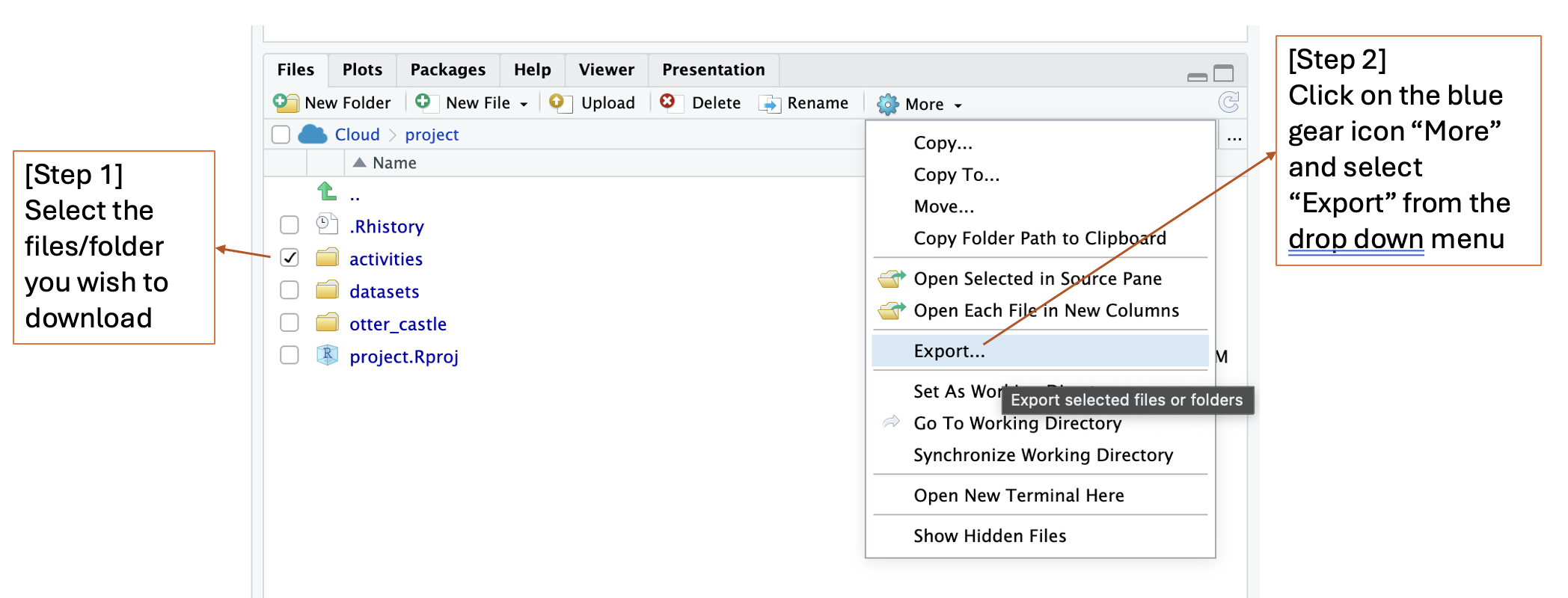
💡 Pro tip: If you don’t select anything, Export will download the current folder you’re viewing.

1. Ice Breaker: Mixed Treasure Bag Sorting Game

Duration: 10 minutes

1.1 Activity: The Great Treasure Sort Competition

🎈 Activity: The Great Treasure Sort Competition

Let’s start with a treasure sort! Your team will get a bag of mixed treasures and a mission.

What you’ll need: A bag or box of mixed items for each team (e.g., colorful tokens, different types of pens, beads, LEGO bricks).

Your Mission:

1. Form teams of 3-4 people. Each team gets one bag.

2. Empty your bag of treasures onto the table.

3. Your challenge: Work together to count how many items you have for each category. For example, your result might be “5 red tokens, 3 blue tokens, and 2 green LEGOs.”

4. 🏆 The first team to get their counts wins!

1.2 Team Reflection

Once you have your counts, think about this:

• What steps did your team take to complete the mission?

• Did you sort the items first? Why?

1.3 Connecting to Code

Guess what? The steps you took are the exact steps data wizards use to wrangle data with code!

• When you sorted items into piles (like all the red things together), you were performing a group_by() operation.

• When you counted the items in each pile, you were doing a summarize().

• If we asked you to find only the pens, you would be using select().

You just acted out a real data analysis workflow! Today, we’ll teach you the spells to do this in R.

2. Let’s Create Our Own Magical Creatures!

Duration: 15 minutes

2.1 Activity: Become a Creature Creator

🎈 Activity: Become a Creature Creator

Now it’s your turn to add to our magical world! We’re going to create a brand new dataset together, with creatures designed by YOU!

Your mission is to fill out this Google Form to invent your own magical creature. Be as creative as you like!

After you submit, you can click “submit another response” to create even more creatures!

https://forms.gle/YmR896E9yC1Zva3KA

Here are the details you’ll get to add about your creatures:

• What is your wizard name?

• What is your magical creature’s name?

• What type of creature is it?

• How old is your creature (please enter number only)?

• On a scale of 1-10, how powerful is its magic?

• Does your creature have wings?

• What is its primary magical element?

• What superpower does this creature has?

What happens next? Once everyone has submitted their creature, I will export the data and upload it to Posit Cloud as a new CSV file. Then, we will use our new data wrangling and visualization spells to explore the world we created together!

3. Data Loading Magic

Duration: 15 minutes (plus Optional 10 minutes for Cleaning)

3.1 Spell 1: Reading CSV Files

Duration: 15 minutes

🎈 Activity: Opening Data Treasure Chests

3.1.1 💡 What is a CSV file?

A CSV (Comma-Separated Values) file is like a super organized spreadsheet saved in a simple text format. Think of it as a list where every piece of information is separated by a comma. It’s a bit like writing a list of your magical creatures and their powers:

Creature_Name, Type, Magic_Power
Sparkle, dragon, 10
Whiskers, fairy, 5
Thunder, phoenix, 9

R can easily read these files to bring data into our magical world!

3.1.2 💡 Understanding File Paths - A Treasure Map for Your Computer!

Before we can load our data, we need to tell R exactly where to find it. Think of a file path as a treasure map that guides R to your file. There are two kinds of maps!

The World Treasure Map (Absolute Path): This is like a full address that can find a treasure from anywhere in the world, but it only works for one specific treasure chest.

• Example: C:/Users/Sky/Sky_documents/Day_3/activities/day03_spell01_loading_data.Rmd

• What it means: This path starts from the very beginning of Sky’s computer’s storage (C:/) and gives every single step to find the file.

• Problem: If I give this map to you, it won’t work! Your computer doesn’t have a folder called Sky, or Sky_documents. It’s too specific to Sky’s computer!

Your Secret Treasure Map (Relative Path): This is like a map that works from a starting point that you both know, the Day_3 folder that you both have!

• Example: "activities/day03_spell01_loading_data.csv"

• What it means: “From right here inside our Day_3 folder, go into the datasets folder, and you’ll find the day03_spell01_loading_data.Rmd file.”

• Why it’s better: This map works for anyone who has the Day_3 folder! When you share your project, your friend can use the same map to find the treasure on their computer.

🎯 Always use relative paths in your R spells! This way, your magic will work on any computer, not just your own.

3.1.3 💡 What does .. mean?

The .. symbol means “go up one level” to the parent folder from where you are currently located.

📁 Example Folder Structure:

🏰 otter_castle
├── 📚 library/
│   ├── 🎣 fish_catching/
│   │   ├── 🐟 salmon/
│   │   └── 🦪 clam/
│   ├── 🔮 magic_spells/
│   │   ├── 🧪 potion_magic/
│   │   └── 🪶 flying_magic/
│   └── 🐾 creatures/
│       ├── 👹 giants/        ← You are **HERE** !
│       ├── 🦄 unicorns/
|       |    └── 🦄 unicorn_data.csv
│       └── 🐱 cats/
└── 🖼️ museums/

🎯 Example: Going Up One Level

If you’re currently in the giants folder and want to access the unicorn_data.csv inside of the unicorns folder:

• Your current location: creatures/giants/

• Target location: creatures/unicorns/

• Magic path: ../unicorns/unicorn_data.csv

✨ Breaking it down:

• .. = “Go up from inside of the giants folder to inside of the creatures folder”

• /unicorns/ = “Then go into the unicorns folder”

• /unicorn_data.csv = “And grab this magical file!”

🎈 Think of it like exploring Otter Castle: You’re in the Giants’ Lair, but the magical unicorn data is in the Unicorns’ Garden next door. You need to go back to the main Creatures Hall first (..), then enter the Unicorns’ Garden (/unicorns/)!

3.1.4 🎈 Try to move around in Oda’s castle yourself!

In R, to find out where you are at currently (which folder are you in), you can use this magic function:

getwd()

To move to a folder that you want to be in, you can use this magic function:

setwd("path/to/your/folder")

🎈 A self- guided tour at Oda’s castle:

📁 Find this spell in Posit Cloud: Look for the file day03_spell01A_castle_navigation.R!

You start at the base of Day 3’s folder. Let’s visit rooms in Oda’s castle in this order:

1. Go to otter_castle/library/creatures/

2. Go back to otter_castle/library/

3. Go into otter_castle/library/fish_catching/

4. Finally, go to otter_castle/museums/

Example:

# Tiny demo (you'll complete the full version in the script!)
getwd()                                  # Where am I now?
setwd("otter_castle/library/creatures") # Move to creatures
getwd()                                  # Confirm where you are
setwd("../")                            # Back to library
getwd()                                  # Confirm where you are

3.1.5 Our own magical creature data:

📁 Find this spell in Posit Cloud: Look for the file day03_spell01_loading_data.Rmd in your project files!

💡 If you are confused about any functions, remember to use the magic of ?!

# Step 1: Load the treasure chest (read the data)
# We'll use the raw form data first (messy on purpose!)
creatures_raw <- read.csv("datasets/creature_of_sky.csv")

# For later, after we clean it, we'll use this:
# creature_data <- read.csv("datasets/creatures.csv")

# Step 2: Peek inside (look at first few rows)
head(creatures_raw)

# Step 3: Peek inside (look at last few rows)
tail(creatures_raw)

# Step 4: Count our treasures (check size)
nrow(creatures_raw)  # how many responses? (how many rows)
ncol(creatures_raw)  # how many details about each response? (how many columns)
dim(creatures_raw)   # how many rows and how many columns?

# Step 5.5: What kind of details do we have? (column names)
print("📝 Columns in our raw creatures data:")
names(creatures_raw)

3.2 Spell 1B: Cleaning Real Data (Optional)

Duration: 10 minutes (Optional)

🎈 Activity: Turn Messy Data into Magic

• Real data from Google Forms is often messy (typos, missing numbers, funny answers).

• We clean the data once, then use the clean file for all other spells.

3.2.1 What did we clean?

• Renamed long form questions to simple column names like creature_name, creature_type, creature_age, magic_power, has_wings

• Turned text data into real numbers (e.g., ages and magic power)

• Fixed has_wings answers to just yes or no

• Removed rows with missing or impossible values (like negative ages)

📁 Find this spell in Posit Cloud: Look for the file day03_spell01B_clean_creatures.R in your project files!

4. Data Wrangling Adventures

Duration: 60 minutes

4.1 Spell 2: The Ultimate Data Toolkit

Duration: 20 minutes

🎈 Activity: Play with our own creatures!

📁 Find this spell in Posit Cloud: Look for the file day03_spell02_data_wrangling.Rmd in your project files!

# Load our data toolbox
library(dplyr)

# First, load your creature data (clean file from 3.2)
creature_data <- read.csv("datasets/creatures.csv")

4.1.1 💡 What is select()?

The select() spell is like choosing which characteristics about your creature you want to look at. Instead of trying to understand every aspect about every single creature at once (their name, age, type, power level, if they have wings), you might select() only 1 or a few characteristics to look at first. You might select() just the creature_name and magic_power to see who’s the strongest. This chooses characteristics (columns) only — it does not remove any creatures (rows); you are still looking at all the creatures but focusing on just their name and power. It helps you focus on only the columns you need and discard irrelevant information.

# SELECT: Pick only the name and type columns (choose features/columns)
creature_basics <- select(creature_data, creature_name, creature_type)
# Un-comment the code below to see the new dataframe
# creature_basics

4.1.2 💡 What is filter()?

The filter() spell keeps only the creatures (rows) that meet your rule. You set a criterion on a characteristic (column), like magic_power >= 80 or type == "dragon". This does not change which characteristics (columns) you see — it does not remove any characteristics (columns); it chooses which rows stay based on your threshold or criteria.

# FILTER: Keep only creatures with wings (choose rows by a rule)
winged_creatures <- filter(creature_data, has_wings == "yes")
# Un-comment the code below to see the new dataframe
# winged_creatures

4.1.3 💡 What is arrange()?

The arrange() spell is like lining up your creatures from shortest to tallest, or weakest to strongest. It sorts your data based on 1 or a few characteristics of the creatures. By default, arrange() sorts your data from smallest to biggest. Use arrange(your_data, desc(column_name)) to sort from biggest to smallest.

# ARRANGE: Sort creatures by age (youngest first)
creatures_by_age <- arrange(creature_data, creature_age)
# Un-comment the code below to see the new dataframe
# creatures_by_age

4.1.4 💡 What is slice()?

The slice() spell picks rows by their position in the table. It’s like choosing creatures from a lineup by their position in the queue. You can grab the first three with slice(1:3), or just the tenth one with slice(10).

# SLICE: Get the top 3 oldest creatures (pick rows by position)
oldest_creatures <- arrange(creature_data, desc(creature_age))
top_3_oldest <- slice(oldest_creatures, 1:3)
# Un-comment the code below to see the new dataframe
# top_3_oldest

4.2 Spell 3: Grouping and Mutating Magic

Duration: 20 minutes

🎈 Activity: Sorting Creatures into Teams

📁 Find this spell in Posit Cloud: Look for the file day03_spell03_grouping.Rmd in your project files!

# GROUP BY and SUMMARIZE: Count each creature type and find their average power

# Step 1: Put creatures into teams by type
by_type <- group_by(creature_data, creature_type)

# Step 2: Ask each team for a report
creature_summary <- summarize(by_type,
                              how_many = n(),
                              average_power = mean(magic_power))
# Un-comment the code below to see the new dataframe
# creature_summary

4.2.1 💡 What is group_by()?

Think of group_by() like sorting your creatures into teams. All the dragons stand together, all the phoenixes together, and so on. This helps us compare teams easily.

4.2.2 💡 What is summarize()?

After the teams are made, summarize() asks each team one clear question and gets one clear answer back. For example: “How many are in your team?” or “What is your team’s average magic power?”

4.2.3 💡 What are n() and mean()?

• n() counts how many are in the team.

• mean() finds the average of a characteristic in the team (like what is the average magic_power of all creatures in the team).

Classify different creatures based on age:

# Add a new column to label creatures as "young" or "old"
creatures_enhanced <- mutate(creature_data,
                             age_category = ifelse(creature_age > 100, "old", "young"))
# Un-comment the code below to see the new dataframe
# creatures_enhanced

4.2.4 💡 What is mutate()?

mutate() creates a brand-new column using the ones you already have. It’s like giving each creature a new label based on a rule.

4.3 Spell 4: Pipeline Magic

Duration: 20 minutes

🎈 Activity: Chaining Commands Like Magic

📁 Find this spell in Posit Cloud: Look for the file day03_spell04_piping.Rmd in your project files!

# Without a pipe, you need lots of steps:
step1 <- filter(creature_data, creature_age > 50)
step2 <- select(step1, creature_name, creature_type, magic_power)
final <- arrange(step2, desc(magic_power))

# With a pipe, you can chain it all together:
magic_pipeline <- creature_data %>%
  filter(creature_age > 50) %>%
  select(creature_name, creature_type, magic_power) %>%
  arrange(desc(magic_power))

# Find the names of the top 3 most powerful winged creatures:
top_winged_creatures <- creature_data %>%
  filter(has_wings == "yes") %>%
  arrange(desc(magic_power)) %>%
  slice(1:3) %>%
  select(creature_name)

4.3.1 💡 What is the Pipe %>%?

The pipe %>% is one of the most magical spells in R! It lets you chain your commands together in a clear, readable way. It takes the result from the step before and “pipes” it directly into the next step.

💡 %>% vs |> in R

• %>% is from the dplyr R package. You get it when you load dplyr.

• |> is the base R pipe (built into R). It works even without loading packages.

• For our class, using %>% with dplyr is perfect. If you ever see |>, it’s doing the same kind of piping job.

Think of it like cooking a meal:

1. Take vegetables %>%

2. Add water %>%

3. Add spices %>%

4. Cook and serve

5. Data Storytelling with Pictures

Duration: 45 minutes

5.1 Spell 5: Histogram Stories

Duration: 15 minutes

🎈 Activity: Shape Detective

5.1.1 💡 What is a Histogram?

A histogram is a picture that shows how your numbers are spread out. Imagine sorting creature ages into boxes (called bins): 0–10, 10–20, 20–30, and so on. Each bar tells you how many creatures are in each box. The bars touch because ages go in order with no gaps. This helps you see the overall shape — are most creatures young, old, or in-between?

📁 Find this spell in Posit Cloud: Look for the file day03_spell05_histograms.Rmd in your project files!

library(ggplot2)

# Create a histogram to see the shape of creature ages
ggplot(creature_data, aes(x = creature_age)) +
  geom_histogram(fill = "purple", color = "black") +
  labs(title = "How Old Are Our Magical Creatures?",
       x = "Age in Years",
       y = "Number of Creatures")+
  theme_minimal() +
  theme(text = element_text(size = 16),
        plot.title = element_text(size = 20),
        axis.title = element_text(size = 18),
        axis.text = element_text(size = 19))

5.2 Spell 6: Scatter Plot Adventures

Duration: 10 minutes

🎈 Activity: Relationship Detective

5.2.1 💡 What is a Scatter Plot?

A scatter plot is the perfect tool for a relationship detective! It helps you see if two things are connected. For example, does a creature who is older have more magic power? Each dot on the plot represents one creature, showing both their age and their magic level. If the dots form a pattern (like going up and to the right), it suggests a relationship!

📁 Find this spell in Posit Cloud: Look for the file day03_spell06_scatter_plots.Rmd in your project files!

# Look for a relationship between age and magic power
ggplot(creature_data, aes(x = creature_age, y = magic_power)) +
  geom_point(size = 3, color = "blue") +
  labs(title = "Do Older Creatures Have More Magic?",
       x = "Age in Years",
       y = "Magic Power Level")+
  theme_minimal() +
  theme(text = element_text(size = 16),
        plot.title = element_text(size = 20),
        axis.title = element_text(size = 18),
        axis.text = element_text(size = 19))

5.3 Spell 7: Bar Chart Champions

Duration: 10 minutes

🎈 Physical Activity: Human Bar Chart:

• Teams line up behind their category signs

• The longest line “wins” - you can see the comparison instantly!

Which group has the most creatures?

5.3.1 💡 What is a Bar Chart?

A bar chart is perfect for comparing different groups (categorical data). Each bar represents a group, and its height shows the count or value. It makes it super easy to see which group is the biggest! Which type of magical creature is most popular? A bar chart will tell you.

📁 Find this spell in Posit Cloud: Look for the file day03_spell07_bar_charts.Rmd in your project files!

# Count each type of creature first
creature_counts <- creature_data %>%
  group_by(creature_type) %>%
  summarize(total = n())

# Create a bar chart
ggplot(creature_counts, aes(x = creature_type, y = total)) +
  geom_col(fill = "orange", color = "black") +
  labs(title = "Which Creature Type is Most Popular?",
       x = "Creature Type",
       y = "Number of Creatures")+
  theme_minimal() +
  theme(text = element_text(size = 16),
        plot.title = element_text(size = 20),
        axis.title = element_text(size = 18),
        axis.text = element_text(size = 19))

Histogram vs. Bar Chart: What’s the Difference?

• Histograms are for numbers that are continuous (like height, score)

• Bar Charts are for comparing separate groups or categories (like creature types: “dragon”, “Fairy”, “Phoenix”).

5.4 🤡 Visualization Crime Alert: Can You Spot What’s Wrong?

Duration: 10 minutes

5.4.1 🚔 Visualization crime 1

Take a look at this real bar plot that was shared when GPT-5 was announced last week by OpenAI:

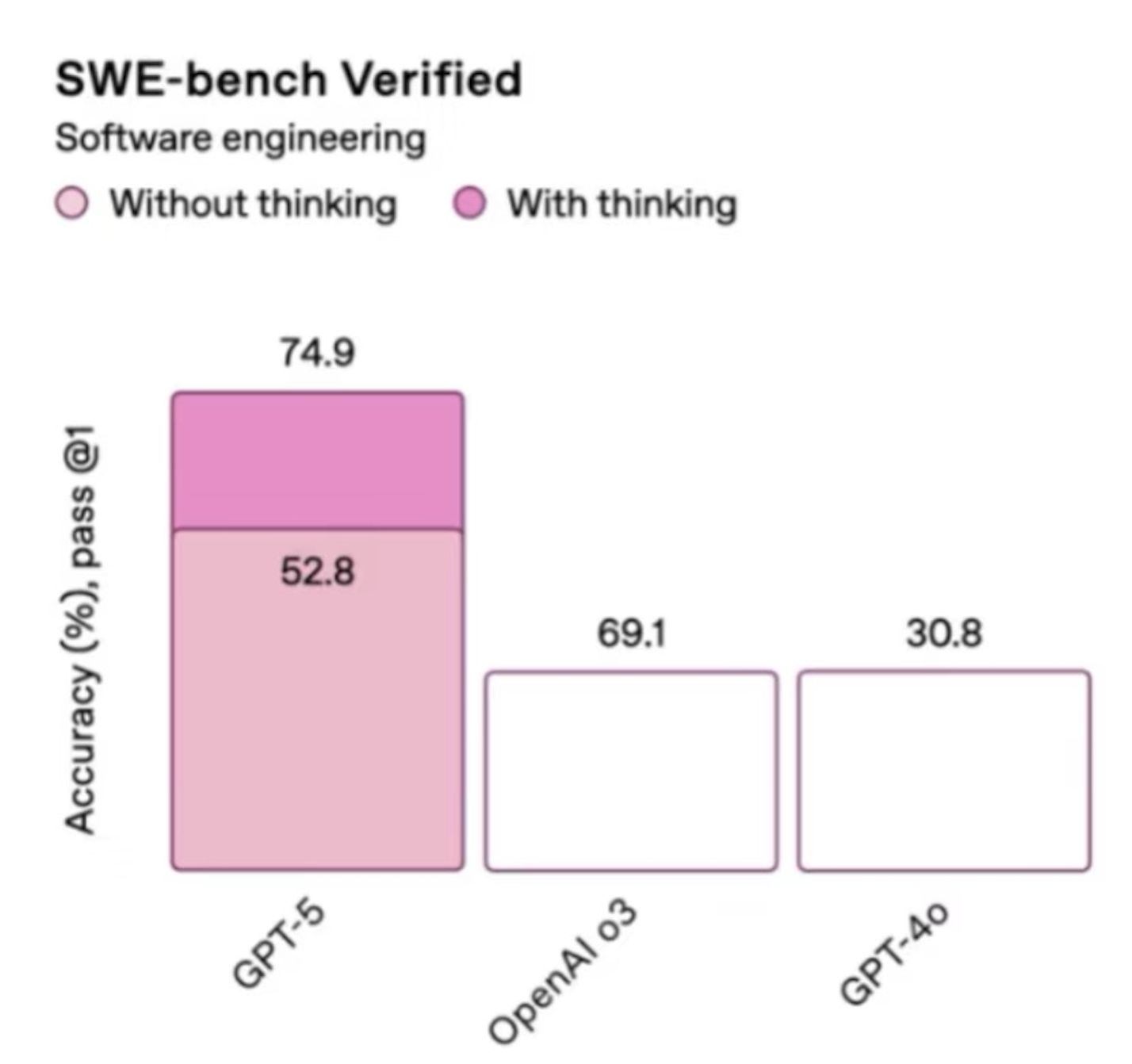
🤔 What’s wrong with this bar plot?

5.4.2 🚔 Visualization crime 2

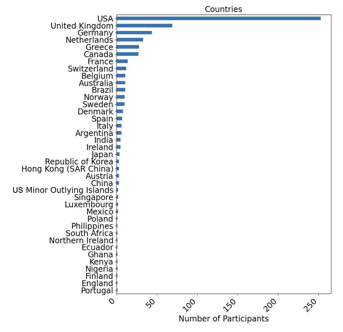
Here is a plot to show “where do participants come from” attending an AI conference

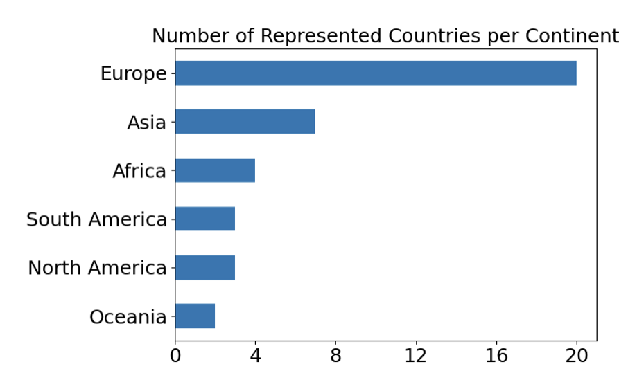
🤔 Where do you think most participants come from according to this plot?

Here is another plot to show where do participants come from attending the SAME AI conference (using the same data set)

🤯 So most people are from the US not Europe! Europe just has more countries than US!

5.4.3 🚔 Visualization crime 3

Here is a plot showing the global temperature changes from 1880 - 2015.

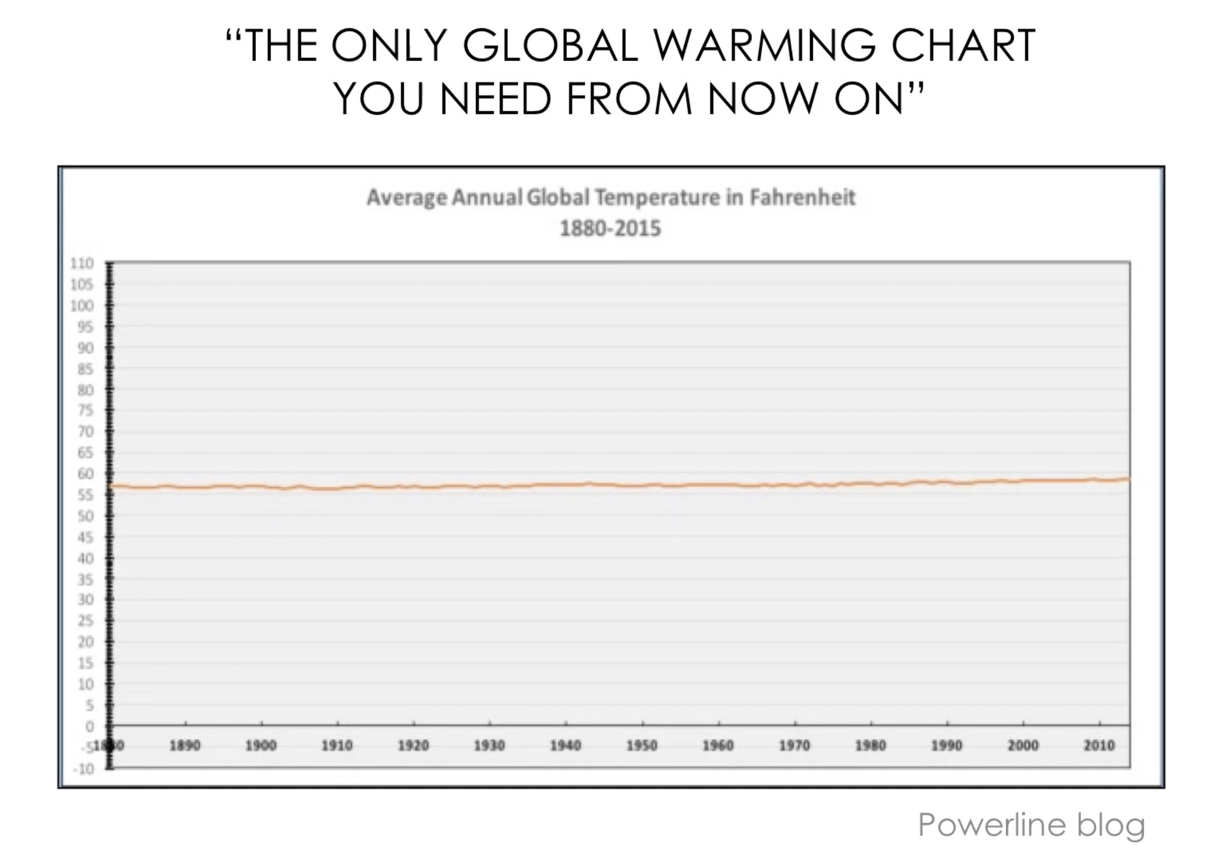
🤔 Looks pretty flat to me! So global warming is not real??

Here is another visualization that is zoomed in, using the same dataset:

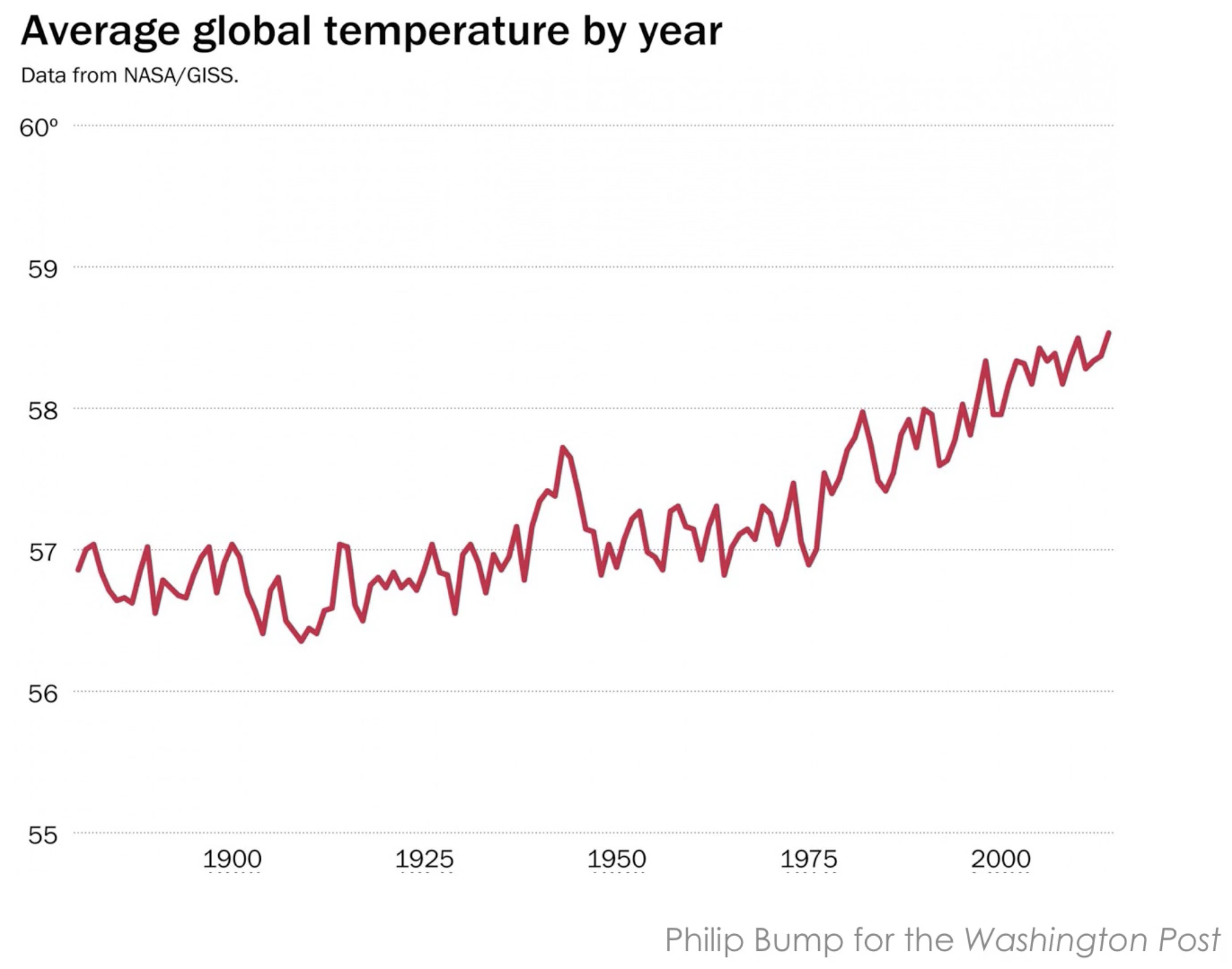
🤯 Global warming is real!!

5.4.4 🚔 Visualization crime 4

Here is a plot from a scientific paper, showing there is a relationship between the prevalence of autisim and the population covergae of measles, mumps, and rubella (MMR) vaccine.

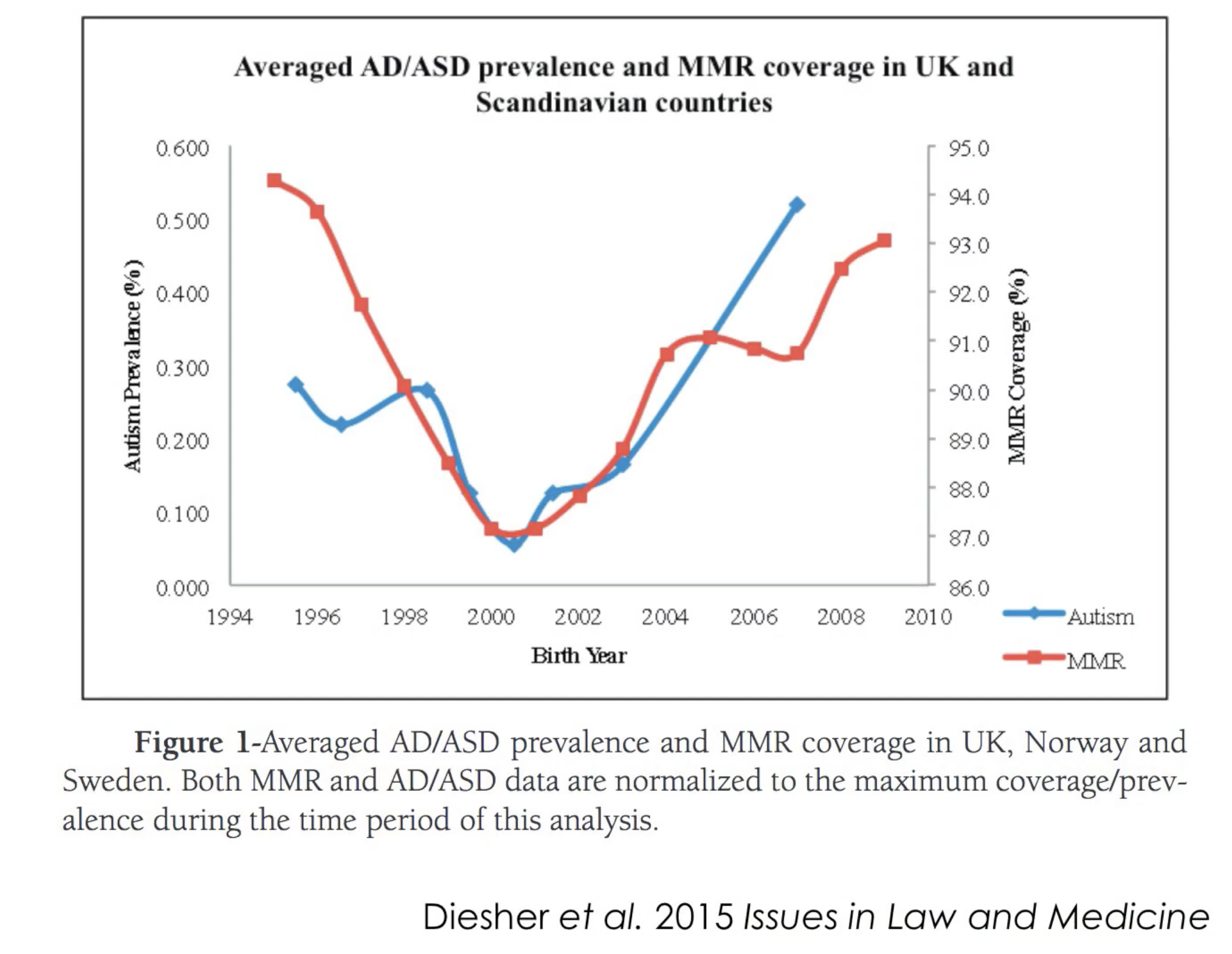
🤔 So does vaccine causes autisim??

Hint: Look at where does both y axis starts? Are they on the same scale?

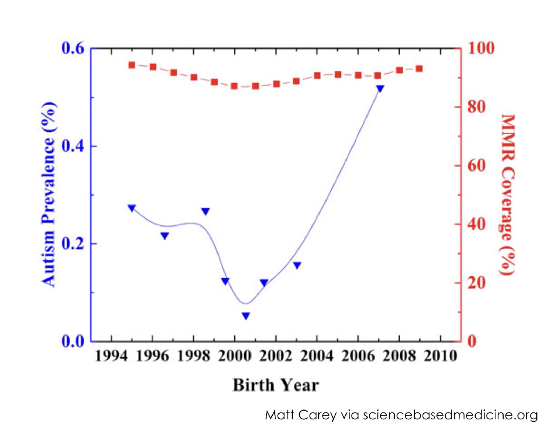
Here is another visualization that is more properly plotted, there is barely any relationship between the 2 lines.

🤯 Vaccine does not cause autisim!! Correlation is also not causation!

6. Team Data Detective Project

Duration: 35 minutes

6.1 Spell 8: Data Mystery Solving

Duration: 35 minutes

📁 Find this spell in Posit Cloud: Start with day03_spell08_team_project.Rmd (overview), then open ONE of:

• day03_spell08A_creatures_project.Rmd (uses creatures.csv)

• day03_spell08B_magical_pets_project.Rmd (uses magical_pets.csv)

• day03_spell08C_creature_sightings_project.Rmd (uses creature_sightings.csv)

• day03_spell08D_magic_school_project.Rmd (uses magic_school_grades.csv)

6.1.1 Activity: Partner Data Investigation

🎈 Activity: Partner Data Investigation

🕵️‍♀️ Mission: Solve a Data Mystery!

Work with a partner to become data detectives! Choose one or many mysteries to solve using our creature datasets:

Mystery Options:

1. Creature Power Mystery (creatures.csv): Which creature type has the highest average magic power? Do winged creatures tend to be more powerful? Are older creatures more magical?

2. Magical Pets Treat Mystery (magical_pets.csv): Which favorite treat is most popular? Do pets who like that treat also tend to have higher magic levels?

3. Creature Sightings Mystery (creature_sightings.csv): Which location has the most creature sightings? What’s the rarest creature spotted?

4. Magic School Mystery (magic_school_grades.csv): Which subject do students struggle with most? Who are the top students?

Your Detective Tools:

• Use select() to pick important clues

• Use filter() to focus on specific evidence

• Use slice() and arrange() to find top/bottom performers

• Use group_by() and summarize() to count and calculate

• Create at least one visualization to show your findings

🎯 Investigation Steps:

1. Load your chosen dataset(s)

2. Explore it with head() and str()

3. Use data wrangling to find clues

4. Create a visualization to tell your story

5. Present your findings to the class!

✨ Challenge: Create the most creative visualization that clearly shows your discovery!

7. 📋 Pro Tips Cheatsheet

7.1 Data Loading Essentials

• read.csv("filename.csv") opens data files like treasure chests

• head(data) shows first 6 rows (peek inside the chest)

• tail(data) shows last 6 rows (peek inside the chest)

• nrow(data) counts how many rows (how many creatures)

• ncol(data) counts how many columns (how many characteristics per creature)

• dim(data) counts both how many rows (first number), and how many columns (second number)

• Always check your data after loading it!

• Use relative paths like "datasets/creatures.csv" so your code works on any computer

• .. means “go up one level” to the parent folder from where you are currently located

• Use getwd() to print current folder that you are in

• Use setwd("path/to/your/folder") to move to a folder you want to be in

7.2 Data Wrangling with dplyr

• library(dplyr) loads an open-source R package with code written by someone else (don’t forget this!).

• select(data, column1, column2) picks specific columns.

• filter(data, condition) keeps only rows that match a rule.

• arrange(data, column) sorts your data (use desc() for biggest first).

• slice(data, 1:5) picks specific rows by their position.

• group_by(data, category) sorts your data into teams.

• summarize(count = n()) calculates a summary for each team (like counting or averaging).

• mutate(data, new_col = calculation) creates new columns.

7.3 Data Cleaning Essentials (from Spell 1B)

• rename() shortens long column names to simple ones (lowercase)

• as.numeric() turns number-like text into real numbers

• gsub() removes unwanted characters from text before converting

• ifelse() helps create clean categories like yes/no

• filter() removes rows with missing or impossible values

• write.csv() saves your cleaned data for everyone to use

7.4 Pipeline Magic

• %>% means “then do this next”, from dplyr package

• |> also means “then do this next”, from base R (do not need to load packages), most of the time it’s interchangable with %>%

• data %>% filter() %>% select() %>% arrange() chains commands together

• Read like instructions: “take data, then filter, then select, then sort”

7.5 Visualization Basics with ggplot2

• library(ggplot2) loads your plotting toolbox (ggplot2 R package).

• geom_histogram() creates histograms, shows the shape of numbers (for continuous data).

• geom_point() creates scatterplots, shows relationships between two variables (characteristics of each data point).

• geom_col() creates bar plot, compares different categories (for categorical data).

• Add titles and labels with labs(title = "My Title").

• Use color = or fill = to make your plots colorful and easier to understand.

8. 🆘 Troubleshooting Cheatsheet

8.1 Data Loading Problems

🐛 Error: “cannot open file”

• What it means: R can’t find a way to walk to your file

• Why it happens: File name is wrong or file isn’t where you think it is (path is wrong)

• The Fix: Check that creatures.csv exists in datasets folder, check spelling exactly

🐛 Error: “creature_data object not found”

• What it means: You’re trying to use creature_data but it doesn’t exist

• Why it happens: Forgot to run the code that loads your creature data

• The Fix: Run the creature_data <- read.csv("datasets/creatures.csv") line first

8.2 Function Problems

🐛 Error: “could not find function”

• What it means: R doesn’t know what select() or filter() means

• Why it happens: Forgot to load the dplyr package

• The Fix: Run library(dplyr) or library(ggplot2) first

🐛 Error: “object ‘creature_name’ not found”

• What it means: Column name (creature_name) doesn’t exist in your creature data

• Why it happens: Typo in column name or your columns are named differently

• The Fix: Check column names with names(creature_data) and fix spelling

8.3 Pipeline Problems

🐛 Pipeline not working

• What it means: Something wrong in the chain of %>% commands

• Why it happens: Forgot to load dplyr, or syntax error in pipeline

• The Fix: Load library(dplyr) first, test each step separately

8.4 Plotting Issues

🐛 “continuous value supplied to discrete scale”

• What it means: Trying to color by a number when ggplot expects categories

• Why it happens: Using color = creature_age instead of color = creature_type

• The Fix: Use categorical variables (like creature_type) for colors

---

💡 Remember: It’s ok to get errors, even your instructor still get error every day! That’s how we leran and grow to be better data scientists!