1. 🚨 Important: Set Your Global Variables First
Before analyzing replacement behavior, configure global variables to match your data structure:
# Configure global variables for your data structure
set_global_cols(
# Time zone
tz = "America/Vancouver",
# Column names in your data files
id_col = "cow",
trans_col = "transponder",
start_col = "start",
end_col = "end",
bin_col = "bin",
dur_col = "duration",
intake_col = "intake",
start_weight_col = "start_weight",
end_weight_col = "end_weight",
# Bin settings
bins_feed = 1:30,
bins_wat = 1:5,
bin_offset = 100
)2. Introduction to Replacement Detection
🦦 Ollie the Otter explains: “Replacement events occur when one animal pushes and displaces another animal that is actively feeding or drinking from a feeding station within a short time window. These social interactions reveal important information about herd dynamics and dominance hierarchies.”
Understanding replacement behavior helps researchers and farm managers:
- Monitor social stress: High replacement rates may indicate social tension
- Identify dominant animals: Animals that frequently replace others
- Affective state: Animals frequently get replaced may experience longitudinal stress
3. Prerequisites
This tutorial assumes completion of previous data processing steps in Tutorial 1: Data Cleaning
4. Data Preparation
# Load cleaned example data
data(clean_comb)
# If you're using your own data from previous tutorials, use this instead:
# clean_feed <- your_cleaned_feed_data # From your cleaning results
# clean_water <- your_cleaned_water_data # From your cleaning results
# Quick peek at our data structure
cat("Feed and water data structure:\n")
#> Feed and water data structure:
head(clean_comb[[1]], 3) # First day, first 3 rows
#> # A tibble: 3 × 11
#> transponder cow bin start end duration
#> <int> <int> <dbl> <dttm> <dttm> <dbl>
#> 1 12448407 6020 1 2020-10-31 00:26:12 2020-10-31 00:27:36 84
#> 2 11954014 4044 1 2020-10-31 01:17:43 2020-10-31 01:22:13 270
#> 3 11954042 4072 1 2020-10-31 01:37:30 2020-10-31 01:37:52 22
#> # ℹ 5 more variables: start_weight <dbl>, end_weight <dbl>, intake <dbl>,
#> # date <date>, rate <dbl>
cat("\nTotal days of feed & water data:", length(clean_comb), "\n")
#>
#> Total days of feed & water data: 25. Understanding Replacement Events
A replacement event is defined as when one animal (actor) takes over a feeding station from another animal (reactor) within a short time threshold. The default threshold of 26 seconds is based on validated research.
Key Components
- Reactor cow: The cow that was replaced (had to leave the bin)
-
Actor cow: The cow that initiated the replacement
(took over the bin)
- Time threshold: Maximum gap between when one cow leaves and another arrives (default: 26 seconds)
- Validation: Events are verified by checking if the actor cow has an “alibi” (was feeding elsewhere when the reactor left)
Detecting Replacement Events
# Process replacement events for all days
replacements <- record_replacement_days(
comb = clean_comb, # Our cleaned feed data
cfg = qc_config(replacement_threshold = 26) # Time gap (seconds) to classify replacement behavior
)
# Examine the first few replacement events
head(replacements[[1]])
#> # A tibble: 6 × 6
#> reactor_cow bin time date actor_cow bout_interval
#> <int> <dbl> <dttm> <date> <int> <Duration>
#> 1 5124 1 2020-10-31 06:07:52 2020-10-31 6020 10s
#> 2 6020 1 2020-10-31 06:09:44 2020-10-31 6069 11s
#> 3 6069 1 2020-10-31 06:12:05 2020-10-31 5124 10s
#> 4 5124 1 2020-10-31 06:13:37 2020-10-31 5067 10s
#> 5 7010 1 2020-10-31 06:20:15 2020-10-31 7018 11s
#> 6 7018 1 2020-10-31 06:20:58 2020-10-31 7010 9s
# Summary of replacement events
cat("Replacement events per day:\n")
#> Replacement events per day:
sapply(replacements, nrow)
#> 2020-10-31 2020-11-01
#> 655 709Each replacement event contains:
-
reactor_cow: ID of the cow that was replaced -
actor_cow: ID of the cow that initiated the replacement -
bin: Feeding/drinking station where the replacement occurred -
time: Timestamp when the replacement happened -
date: Date of the event -
bout_interval: Time gap between when the reactor left and actor entered the bin
6. Analyzing Replacement Patterns
Most Active cows
# Combine all days for analysis
all_replacements <- do.call(rbind, replacements)
# cows that most frequently replace others (actors)
top_actors <- all_replacements |>
dplyr::count(actor_cow, sort = TRUE, name = "times_replaced_others") |>
head(5)
cat("Top 10 cows that most frequently displace others:\n")
#> Top 10 cows that most frequently displace others:
print(top_actors)
#> # A tibble: 5 × 2
#> actor_cow times_replaced_others
#> <int> <int>
#> 1 6050 65
#> 2 5124 61
#> 3 5120 60
#> 4 5058 55
#> 5 5042 52
# cows that are most frequently replaced (reactors)
top_reactors <- all_replacements |>
dplyr::count(reactor_cow, sort = TRUE, name = "times_replaced") |>
head(5)
cat("\nTop 10 cows that are most frequently displaced:\n")
#>
#> Top 10 cows that are most frequently displaced:
print(top_reactors)
#> # A tibble: 5 × 2
#> reactor_cow times_replaced
#> <int> <int>
#> 1 7018 57
#> 2 5042 50
#> 3 7027 49
#> 4 7030 46
#> 5 5123 43Replacement Timing Patterns
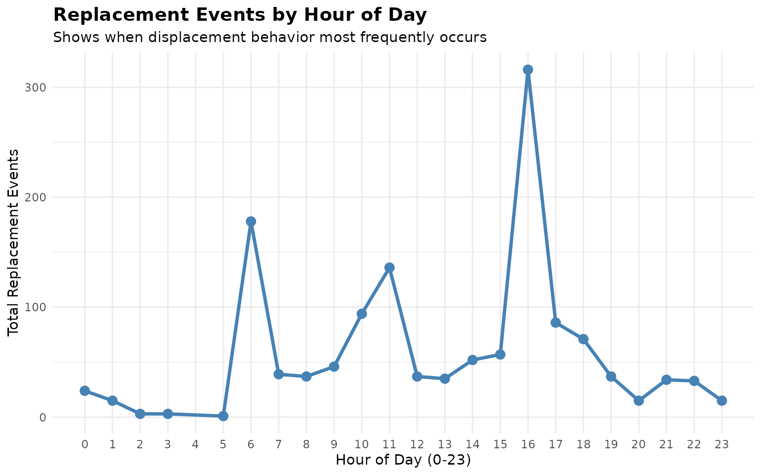
# Analyze replacement timing throughout the day
all_replacements$hour <- lubridate::hour(all_replacements$time)
hourly_replacements <- all_replacements |>
dplyr::count(hour, name = "replacement_count")
cat("Replacement events by hour of day:\n")
#> Replacement events by hour of day:
print(hourly_replacements)
#> # A tibble: 23 × 2
#> hour replacement_count
#> <int> <int>
#> 1 0 24
#> 2 1 15
#> 3 2 3
#> 4 3 3
#> 5 5 1
#> 6 6 178
#> 7 7 39
#> 8 8 37
#> 9 9 46
#> 10 10 94
#> # ℹ 13 more rowsVisualize Replacement Patterns
# Visualize replacement events by hour
ggplot(hourly_replacements, aes(x = hour, y = replacement_count)) +
geom_line(color = "steelblue", linewidth = 1.2) +
geom_point(color = "steelblue", size = 3) +
scale_x_continuous(breaks = 0:23) +
labs(
title = "Replacement Events by Hour of Day",
subtitle = "Shows when displacement behavior most frequently occurs",
x = "Hour of Day (0-23)",
y = "Total Replacement Events"
) +
theme_minimal() +
theme(
plot.title = element_text(size = 14, face = "bold"),
panel.grid.minor.x = element_blank()
)
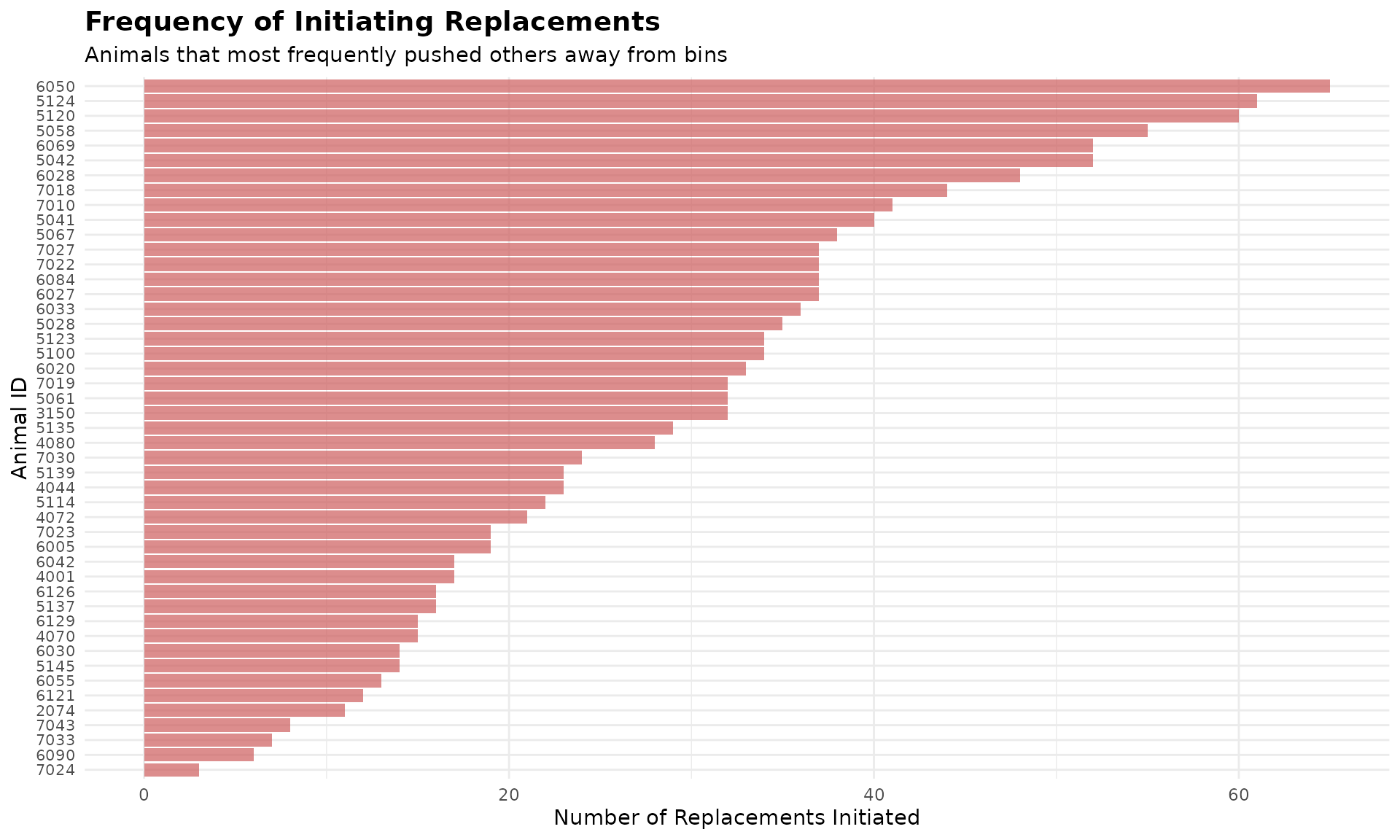
# Visualize top 50 most active displacing animals
top_50_actors <- head(all_replacements |>
dplyr::count(actor_cow, sort = TRUE, name = "times_replaced_others"), 50)
ggplot(top_50_actors, aes(x = reorder(actor_cow, times_replaced_others), y = times_replaced_others)) +
geom_bar(stat = "identity", fill = "indianred", alpha = 0.7) +
coord_flip() +
labs(
title = "Frequency of Initiating Replacements",
subtitle = "Animals that most frequently pushed others away from bins",
x = "Animal ID",
y = "Number of Replacements Initiated"
) +
theme_minimal() +
theme(
axis.text.y = element_text(size = 8),
plot.title = element_text(size = 14, face = "bold")
)
7. Summary
This tutorial demonstrated replacement detection for understanding social dynamics:
Event detection: Identified and validated replacement events using time thresholds
Pattern analysis: Analyzed which cows are most active in displacement behavior
Timing insights: Examined when most replacement events occur throughout the day
8. Code Cheatsheet
#' Copy and modify these code blocks for your own analysis!
# ---- SETUP: Global Variables (REQUIRED FIRST!) ----
library(moo4feed)
library(ggplot2)
library(dplyr)
# Set up your column names and timezone (modify these!)
set_global_cols(
# Time zone
tz = "America/Vancouver",
# Column names in your data files
id_col = "cow",
trans_col = "transponder",
start_col = "start",
end_col = "end",
bin_col = "bin",
dur_col = "duration",
intake_col = "intake",
start_weight_col = "start_weight",
end_weight_col = "end_weight",
# Bin settings
bins_feed = 1:30,
bins_wat = 1:5,
bin_offset = 100
)
# ---- STEP 1: Load Your Data ----
# Load your cleaned data
data(clean_comb)
# Or use your own cleaned data from previous tutorials:
# clean_comb <- your_cleaned_comb_data
# ---- STEP 2: Detect Replacement Events ----
# Process replacement events for all days
replacements <- record_replacement_days(
comb = clean_comb, # Your cleaned feed/water or both feed + water data
cfg = qc_config(replacement_threshold = 26) # Time gap (seconds) to classify replacement behavior
)
# Examine the first few replacement events
head(replacements[[1]])
# Summary of replacement events
cat("Replacement events per day:\n")
sapply(replacements, nrow)
# ---- STEP 3: Analyze Replacement Patterns ----
# Combine all days for analysis
all_replacements <- do.call(rbind, replacements)
# Animals that most frequently replace others (actors)
top_actors <- all_replacements |>
dplyr::count(actor_cow, sort = TRUE, name = "times_replaced_others") |>
head(5)
cat("Top cows that most frequently displace others:\n")
print(top_actors)
# Animals that are most frequently replaced (reactors)
top_reactors <- all_replacements |>
dplyr::count(reactor_cow, sort = TRUE, name = "times_replaced") |>
head(5)
cat("\nTop cows that are most frequently displaced:\n")
print(top_reactors)
# Analyze replacement timing throughout the day
all_replacements$hour <- lubridate::hour(all_replacements$time)
hourly_replacements <- all_replacements |>
dplyr::count(hour, name = "replacement_count")
cat("\nReplacement events by hour of day:\n")
print(hourly_replacements)
# ---- STEP 4: Visualize Results ----
# Replacement events by hour
ggplot(hourly_replacements, aes(x = hour, y = replacement_count)) +
geom_line(color = "steelblue", linewidth = 1.2) +
geom_point(color = "steelblue", size = 3) +
scale_x_continuous(breaks = 0:23) +
labs(
title = "Replacement Events by Hour of Day",
subtitle = "Shows when displacement behavior most frequently occurs",
x = "Hour of Day (0-23)",
y = "Total Replacement Events"
) +
theme_minimal() +
theme(
plot.title = element_text(size = 14, face = "bold"),
panel.grid.minor.x = element_blank()
)
# Most active displacing animals bar plot
top_50_actors <- head(all_replacements |>
dplyr::count(actor_cow, sort = TRUE, name = "times_replaced_others"), 50)
ggplot(top_50_actors, aes(x = reorder(actor_cow, times_replaced_others), y = times_replaced_others)) +
geom_bar(stat = "identity", fill = "indianred", alpha = 0.7) +
coord_flip() +
labs(
title = "Frequency of Initiating Replacements",
subtitle = "Animals that most frequently pushed others away from bins",
x = "Animal ID",
y = "Number of Replacements Initiated"
) +
theme_minimal() +
theme(
axis.text.y = element_text(size = 8),
plot.title = element_text(size = 14, face = "bold")
)