DSCI 512 Lecture 4 : Stacks, Queues, and Graph Searches
Sky (Kehan) Sheng
Housekeeping 🏠
- Cheatsheet 1 submission is open.
- Section 004 lab today is at LIFE 2402
- Quiz 1: Next Tuesday to Friday
- Make sure you book a slot for all 4 quizzes.
- The 512 quiz has both multiple choice and coding question.
- Syllabus: lectures 1 to 4 (please review all the material in the lecture notes)
- We will NOT test about Trees in the quiz, and will not discuss Trees in the lecture this week.
Sparse matrices, continued 🦦
Image generated by OpenAI GPT-image-2.5-sunburst
Build a matrix from triples: COO
COO (COOrdinate format, also called triplet format): for every non-zero, store its row, its column and its value.
{
  // Draw only: the triples and the highlights were computed in Python (coo_view).
  const s = coo_view.steps[coo_k];
  const header = html`<tr><th></th>${coo_view.col_labels.map(h => html`<th>${h}</th>`)}</tr>`;
  const rows = s.rows.map((r, i) => html`<tr class="${r.cls}"><th>row ${i}</th>
      ${r.cells.map(c => html`<td class="${c.cls}">${c.v}</td>`)}</tr>`);
  const boxes = items => items.map(b =>
    html`<div class="ds-box ${b.cls}">${b.label}<span class="sq-tag below">${b.tag}</span></div>`);
  return html`<div class="adj-wrap csr-wrap">
      <div class="adj-panel">
        ${s.arrays.map(a => html`<div class="ds-row csr"><span class="csr-name">${a.name}</span>${boxes(a.boxes)}</div>`)}
        <div class="ds-caption">what COO stores (small numbers: triple number)</div></div>
      <div class="adj-panel"><table class="adj-table">${header}${rows}</table>
        <div class="ds-caption">the matrix we build</div></div>
    </div>
    <div class="ojs-readout">${s.say.join(" ")}</div>`;
}
How CSR stores a matrix in a compressed way
CSR (Compressed Sparse Row). The matrix does not need to be square: this one has 4 rows and 3 columns.
{
  // Draw only: the arrays and the highlights were computed in Python (csr_view).
  const s = csr_view.steps[csr_row];
  const header = html`<tr><th></th>${csr_view.col_labels.map(h => html`<th>${h}</th>`)}</tr>`;
  const rows = s.rows.map((r, i) => html`<tr class="${r.cls}"><th>row ${i}</th>
      ${r.cells.map(c => html`<td class="${c.cls}">${c.v}</td>`)}</tr>`);
  const nnzRows = s.nnz.map(r => html`<tr class="${r.cls}"><td>${r.v}</td></tr>`);
  const boxes = items => items.map(b =>
    html`<div class="ds-box ${b.cls}">${b.label}<span class="sq-tag below">${b.tag}</span></div>`);
  return html`<div class="adj-wrap csr-wrap">
      <div class="adj-panel"><table class="adj-table">${header}${rows}</table>
        <div class="ds-caption">the matrix</div></div>
      <div class="adj-panel"><table class="adj-table">
          <tr><th>non-zeros</th></tr>${nnzRows}</table>
        <div class="ds-caption">count per row</div></div>
      <div class="adj-panel">
        <div class="ds-row csr"><span class="csr-name">data</span>${boxes(s.data)}</div>
        <div class="ds-row csr"><span class="csr-name">indices</span>${boxes(s.indices)}</div>
        <div class="ds-row csr"><span class="csr-name">indptr</span>${boxes(s.indptr)}</div>
        <div class="ds-caption">what CSR stores (small numbers: position in the array)</div></div>
    </div>
    <div class="ojs-readout">${s.say.join(" ")}</div>`;
}
Sparse matrices: CSR in code
From CSR back to the matrix
Given only data, indices and indptr, can we get the matrix back?
{
  // Draw only: every highlight, cell and sentence was computed in Python (rebuild_steps).
  const s = rebuild_steps[rebuild_step];
  const header = html`<tr><th></th>${csr_view.col_labels.map(h => html`<th>${h}</th>`)}</tr>`;
  const rows = s.rows.map((r, i) => html`<tr class="${r.cls}"><th>row ${i}</th>
      ${r.cells.map(c => html`<td class="${c.cls}">${c.v}</td>`)}</tr>`);
  const boxes = items => items.map(b =>
    html`<div class="ds-box ${b.cls}">${b.label}<span class="sq-tag below">${b.tag}</span></div>`);
  const say = s.say.map(([t, cls]) => html`<span class="${cls}">${t}</span>`);
  const work = s.work.map(w => html`<tr class="${w.cls}"><td class="code">${w.formula}</td>
      <td class="gives">${w.gives}</td><td class="code value">${w.value}</td></tr>`);
  return html`<div class="ojs-readout"><span class="sq-count">${s.count}</span> ${say}</div>
    <div class="adj-wrap csr-wrap">
      <div class="adj-panel">
        <div class="ds-row csr"><span class="csr-name">data</span>${boxes(s.data)}</div>
        <div class="ds-row csr"><span class="csr-name">indices</span>${boxes(s.indices)}</div>
        <div class="ds-row csr"><span class="csr-name">indptr</span>${boxes(s.indptr)}</div>
        <div class="ds-caption">what CSR stores (small numbers: position in the array)</div></div>
      <div class="adj-panel"><table class="adj-table">${header}${rows}</table>
        <div class="ds-caption">the matrix, rebuilt</div></div>
    </div>
    <div class="adj-wrap"><table class="adj-table csr-work">
      <tr><th>formula</th><th>gives</th><th>${s.work_head}</th></tr>${work}</table></div>`;
}
Rebuild it in code
The same three steps per row, as a loop:
scipy does this for you: x.toarray().
Working with sparse matrices
Many NumPy operations work. Can we add up each row without building the dense matrix?
- Row 0 holds 5 and 1, so its total should be 6.
- Row 1 is empty, so its total is 0.
- Row 2 holds 2 and 3, so its total should be 5.
- Row 3 holds 4, so its total is 4.
Tricks in Python
axis = 1VSaxis = 0axissays which direction to add up.axis=1collapses the columns, so you get one total per row.axis=0collapses the rows, so you get one total per column.
- Use
x[i, j]to access the element in rowiand columnj, notx[i][j].
Rows vs columns: CSR and CSC
CSR is stored row by row. CSC (Compressed Sparse Column) is the same idea, column by column.
The code below has 2 functions, one pulls out 200 rows, and the other pulls out 200 columns. We time how long it takes when we use CSR VS CSC.
G_10k = nx.fast_gnp_random_graph(10_000, 0.0025, seed=512)   # 10,000 users
csr = nx.adjacency_matrix(G_10k)
csc = csr.tocsc()          # convert once, before any loop

def get_rows(m, k=200):
    for i in range(k):
        m[[i], :]          # row i, all columns

def get_cols(m, k=200):
    for j in range(k):
        m[:, [j]]          # all rows, column j

times = {}
for name, m in [("CSR", csr), ("CSC", csc)]:
    times[name, "rows"] = timeit.timeit(lambda: get_rows(m), number=1)
    times[name, "columns"] = timeit.timeit(lambda: get_cols(m), number=1)
    print(f"{name}: 200 rows {times[name, 'rows'] * 1e3:6.1f} ms,  200 columns {times[name, 'columns'] * 1e3:6.1f} ms")
CSR: 200 rows 8.7 ms, 200 columns 68.3 ms
CSC: 200 rows 68.6 ms, 200 columns 6.1 msEach format is fast in its own direction
// Draw only: every time was measured in Python (timing_chart).
Plot.plot({
  width: 880, height: 220, marginLeft: 170, marginRight: 90, marginBottom: 46,
  style: {fontSize: "16px", background: "transparent"},
  x: {label: "milliseconds →", labelAnchor: "center", grid: true},
  y: {label: null, domain: timing_chart.bars},
  color: {domain: timing_chart.order, range: ["#2a78d6", "#eb6834"], legend: true, swatchSize: 16},
  marks: [
    Plot.barX(timing_chart.rows, {y: "bar", x: "ms", fill: "what", rx: 4}),
    Plot.text(timing_chart.rows, {y: "bar", x: "ms", text: "label",
                                  dx: 8, textAnchor: "start", fontWeight: "bold"}),
    Plot.ruleX([0])
  ]
})Which one should I use?
| Your situation | Use |
|---|---|
| Small matrix, or more than about 10% non-zeros | dense matrix |
| Linear algebra calculation (e.g., full factorizations or eigendecompositions) | dense matrix |
| Large matrix, with lots of zeros | sparse matrix |
| Building it one entry at a time | COO, then convert |
| Mostly reading rows (most of scikit-learn; matrix-vector multiplication) | CSR |
| Mostly reading columns (extracting all values in certain features for a machine learning model) | CSC |
| Look up edges or if two vertices are connected | adjacency matrix |
| Graph search: visit each node’s neighbours | adjacency list, or CSR |
Density thresholds: MLX sparse, Performance guide
Sparse data is everywhere
- Natural language processing: a document-term matrix, one row per document, one column per word. Each document uses only a tiny fraction of the vocabulary.
- One-hot encoding: scikit-learn’s
OneHotEncoderreturns a sparse matrix by default. - Recommendation systems: a user-item matrix, one row per user, one column per item. Each user interacts with only a few items.
Screenshot: DSCI 571 lecture notes, Chapter 4 · Examples: AskPython, SciPy sparse
Word counts are sparse
Example adapted from AskPython, SciPy sparse
Stacks and queues
You are writing an Instagram post with a few photos. Which data structure we should use for the “Undo” button? Which one to use for the “Upload” button? 🤔
Image generated by OpenAI GPT-image-2.5-sunburst
Stack and queue
Stack: LIFO
Last In, First Out
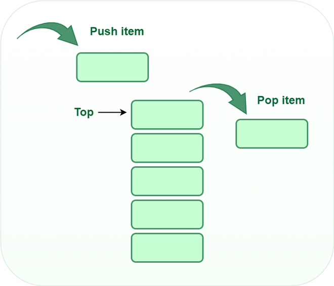
Undo while you edit. Every edit goes on top, and undo takes off the most recent one.
Queue: FIFO
First In, First Out
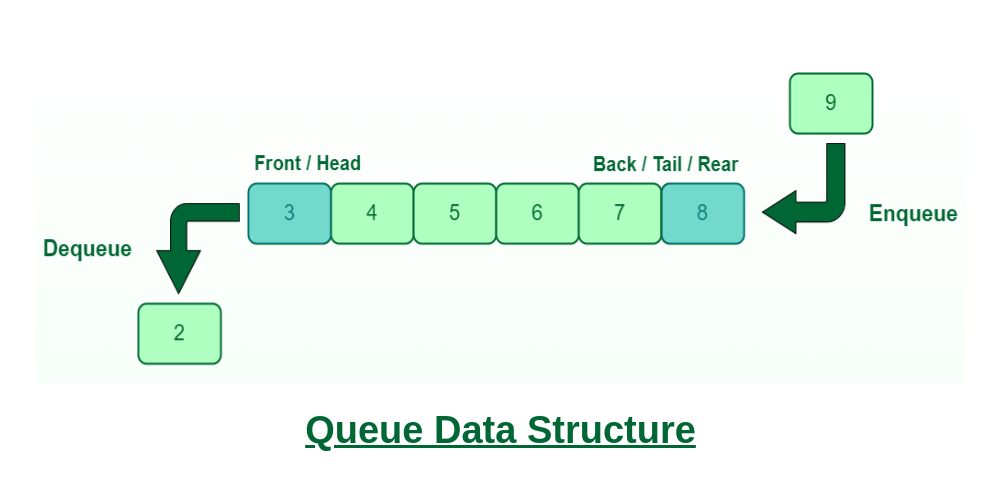
The upload queue. Each photo joins the back, and the server takes the one that has waited longest.
Both add at the back. They differ only in which end you take from.
How a stack works: last in, first out
{
  // Draw only: every box, colour and sentence was computed in Python (stack_steps).
  const s = stack_steps[stack_step];
  const ops = s.ops.map(o => html`<div class="sq-op ${o.cls}">${o.label}</div>`);
  const boxes = s.boxes.map(b =>
    html`<div class="ds-box ${b.cls}">${b.label}<span class="sq-tag right">${b.tag}</span></div>`);
  const out = s.out_so_far.map(label => html`<div class="ds-box out">${label}</div>`);
  return html`<div class="sq-ops">${ops}</div>
    <div class="sq-say"><span class="sq-count">${s.count}</span>
      <span class="sq-verb ${s.verb_cls}">${s.verb}</span> ${s.say}</div>
    <div class="sq-stage">
      <div class="sq-lift">
        <div class="ds-box ${s.removed_cls}">${s.removed}</div>
        <div class="sq-ends">
          <span class="sq-arrow add ${s.add_cls}">⬇ add</span>
          <span class="sq-arrow remove ${s.remove_cls}">⬆ remove</span>
        </div>
        <div class="sq-stack">${boxes}</div>
        <div class="ds-caption">undo history</div>
      </div>
      <div class="sq-tray">
        <div class="ds-caption">came out, in order</div>
        <div class="ds-row center">${out.length ? out : html`<span class="ds-caption">nothing yet</span>`}</div>
      </div>
    </div>`;
}How a queue works: first in, first out
{
  // Draw only: every box, colour and sentence was computed in Python (queue_steps).
  const s = queue_steps[queue_step];
  const ops = s.ops.map(o => html`<div class="sq-op ${o.cls}">${o.label}</div>`);
  const boxes = s.boxes.map(b =>
    html`<div class="ds-box ${b.cls}">${b.label}<span class="sq-tag below">${b.tag}</span></div>`);
  const out = s.out_so_far.map(label => html`<div class="ds-box out">${label}</div>`);
  return html`<div class="sq-ops">${ops}</div>
    <div class="sq-say"><span class="sq-count">${s.count}</span>
      <span class="sq-verb ${s.verb_cls}">${s.verb}</span> ${s.say}</div>
    <div class="sq-line">
      <div class="sq-exit"><div class="ds-box ${s.removed_cls}">${s.removed}</div></div>
      <span class="sq-arrow remove ${s.remove_cls}">⬅ remove<br><small>front</small></span>
      <div class="sq-queue">${boxes}</div>
      <span class="sq-arrow add ${s.add_cls}">⬅ add<br><small>back</small></span>
    </div>
    <div class="ds-caption">upload queue</div>
    <div class="sq-tray">
      <div class="ds-caption">came out, in order</div>
      <div class="ds-row center">${out.length ? out : html`<span class="ds-caption">nothing yet</span>`}</div>
    </div>`;
}Stack in code
The top of the stack is the end of the list.
append and pop() both work at the end of a list: \(O(1)\), nothing else moves.
Try it: a stack
Queue in code
The only change from Stack: take from the front of the list.
Try it: a queue
⚠️ list.pop(0) is slow
So we use deque! collections.deque (“deck”, a double-ended queue) adds and removes at both ends in \(O(1)\): append to join the back, popleft to leave the front.
n = 100_000

def empty_list_queue(n):
    q = list(range(n))
    while q:
        q.pop(0)        # O(n) each time: shift everything left

def empty_deque(n):
    q = deque(range(n))
    while q:
        q.popleft()     # O(1) each time

t_list = timeit.timeit(lambda: empty_list_queue(n), number=1)
t_deque = timeit.timeit(lambda: empty_deque(n), number=1)
print(f"list.pop(0):     {t_list * 1e3:8.1f} ms")
print(f"deque.popleft(): {t_deque * 1e3:8.1f} ms   ({t_list / t_deque:,.0f}x faster)")
list.pop(0): 483.8 ms
deque.popleft(): 4.8 ms (100x faster)Demonstration comparing list.pop(0) and deque.popleft()
A list keeps its items in slots 0, 1, 2, … with no gaps. What happens when the front one leaves?
{
  // Draw only: every box, count and sentence was computed in Python (shift_steps).
  const s = shift_steps[shift_step];
  const boxes = items => items.map(b =>
    html`<div class="ds-box ${b.cls}">${b.label}<span class="sq-tag below">${b.tag}</span></div>`);
  const say = s.say.map(([t, cls]) => html`<span class="${cls}">${t}</span>`);
  return html`<div class="ojs-readout"><span class="sq-count">${s.count}</span> ${say}</div>
    <div class="adj-wrap"><div class="adj-panel">
      <div class="ds-row csr shift"><span class="csr-name">list</span>${boxes(s.list)}</div>
      <div class="ds-row csr shift"><span class="csr-name">deque</span>${boxes(s.deque)}</div>
      <div class="ds-caption">orange: moved one slot left (small numbers: slot)</div>
    </div></div>`;
}Emptying a queue of 100,000 items
// Draw only: both times were measured in Python (deque_chart).
Plot.plot({
  width: 860, height: 200, marginLeft: 150, marginRight: 110, marginTop: 20, marginBottom: 46,
  style: {fontSize: "16px", background: "transparent"},
  x: {label: "milliseconds to empty the whole queue →", labelAnchor: "center", grid: true,
      domain: deque_chart.x_domain},
  y: {label: null, domain: deque_chart.order},
  color: {domain: deque_chart.kinds, range: ["#eb6834", "#2a78d6"], legend: true, swatchSize: 16},
  marks: [
    Plot.barX(deque_chart.rows, {y: "how", x: "ms", fill: "kind", rx: 4}),
    Plot.text(deque_chart.rows, {y: "how", x: "ms", text: "bar_label",
                                 dx: 8, textAnchor: "start", fontWeight: "bold"}),
    Plot.ruleX([0])
  ]
})| structure | insert | delete | search | use it when |
|---|---|---|---|---|
| stack (LIFO) | \(O(1)\) push | \(O(1)\) pop | \(O(n)\) | most recent first: undo, back button |
| queue (FIFO) | \(O(1)\) push | \(O(1)\) with deque |
\(O(n)\) | oldest first: upload queues |
Searching in a graph 🔍
How does LinkedIn know ada is your “3rd” level connection?
You search LinkedIn for a data scientist named ada. Next to her name: 3rd.
You have never met ada. LinkedIn has about 1 billion members.

How does LinkedIn know she is 3rd, and not 2nd or 4th?
Image generated by OpenAI GPT-image-2.5-sunburst · Member count: LinkedIn, About us
Breadth-first search: search in rings
{
  // Draw only: the search was run in Python (bfs_run); every colour, label and box comes from there.
  const s = bfs_run.steps[bfs_step];
  const fill = {now: "#eb6834", path: "#eb6834", done: "#2a78d6", waiting: "#a9c8ef", other: "#b8b6b0"};
  const stroke = {path: "#eb6834", found: "#2a78d6", base: "#d9d8d4"};
  const nodes = li_layout.nodes.map((d, i) => ({...d, role: s.node_roles[i], label: s.labels[i]}));
  const edges = li_layout.edges.map((d, i) => ({...d, role: s.edge_roles[i]}));
  const boxes = s.boxes.map(b => html`<div class="ds-box ${b.cls}">${b.label}</div>`);
  return html`<div class="ojs-readout"><span class="sq-count">${s.count}</span> ${s.say}</div>
    ${Plot.plot({
      width: 860, height: 300, margin: 14,
      style: {fontSize: "16px", background: "transparent"},
      x: {axis: null, domain: li_layout.x_domain}, y: {axis: null, domain: li_layout.y_domain},
      marks: [
        Plot.link(edges, {x1: "x1", y1: "y1", x2: "x2", y2: "y2", stroke: d => stroke[d.role],
                          strokeWidth: d => d.role === "base" ? 2 : 4}),
        Plot.dot(nodes, {x: "x", y: "y", r: 13, fill: d => fill[d.role], stroke: "white", strokeWidth: 2}),
        Plot.text(nodes, {x: "x", y: "y", text: "label", dy: -23, fontWeight: "bold"})
      ]
    })}
    <div class="ds-row center"><span class="ds-caption">${s.box_caption}</span>
      ${boxes.length ? boxes : html`<span class="ds-caption">empty</span>`}</div>`;
}BFS in code
def bfs_connected(g, start, goal, verbose=False):
    to_visit = deque([start])   # a queue holding just the start node
    visited = {start}           # nodes we have already put in the queue

    while to_visit:                    # while the queue is not empty
        node = to_visit.popleft()      # take the OLDEST node, from the front
        if verbose:
            print("At node", node)
        if node == goal:
            return True
        for neighbour in g.neighbors(node):
            if neighbour not in visited:
                visited.add(neighbour)
                to_visit.append(neighbour)   # join the back of the queue

return False # the queue ran out and we never reached goalTry it: BFS
BFS finds shortest paths
- BFS visits every 1st before any 2nd, every 2nd before any 3rd. So the first time it reaches a node, it used a shortest path.
- That is how LinkedIn’s “3rd” works, and how
nx.shortest_path_lengthworks on an unweighted graph.
The algorithm
- Put the start node in a “to visit” list.
- Take a node out and visit it.
- Add its neighbours to the list, unless we have already seen them.
- Repeat until the list is empty.
The only real choice is which node to take out next:
| “to visit” list is a… | take out… | search |
|---|---|---|
queue (deque, popleft) |
the oldest node | breadth-first search (BFS) |
stack (list, pop) |
the newest node | depth-first search (DFS) |
iClicker: how fast is BFS?
A graph with \(V\) nodes and \(E\) edges, stored as an adjacency list. Time complexity of BFS in the worst case?
- (A) \(O(V)\)
- (B) \(O(E)\)
- (C) \(O(V + E)\)
- (D) \(O(V^2)\)
- Answer: C. Each node goes in and out of the queue once: \(O(V)\). Looping over neighbours adds up to every degree, \(2E\): \(O(E)\).
- Space: \(O(V)\). The queue and the
visitedset each hold at most \(V\) nodes.
Question: a list as the queue?
What if BFS used a plain list, with list.pop(0) instead of deque.popleft()?
pop(0)is \(O(V)\), called up to \(V\) times: \(O(V^2 + E)\).
Depth-first search: go deep first
{
  // Draw only: the search was run in Python (dfs_run); every colour, label and box comes from there.
  const s = dfs_run.steps[dfs_step];
  const fill = {now: "#eb6834", path: "#eb6834", done: "#2a78d6", waiting: "#a9c8ef", other: "#b8b6b0"};
  const stroke = {path: "#eb6834", found: "#2a78d6", base: "#d9d8d4"};
  const nodes = li_layout.nodes.map((d, i) => ({...d, role: s.node_roles[i], label: s.labels[i]}));
  const edges = li_layout.edges.map((d, i) => ({...d, role: s.edge_roles[i]}));
  const boxes = s.boxes.map(b => html`<div class="ds-box ${b.cls}">${b.label}</div>`);
  return html`<div class="ojs-readout"><span class="sq-count">${s.count}</span> ${s.say}</div>
    ${Plot.plot({
      width: 860, height: 300, margin: 14,
      style: {fontSize: "16px", background: "transparent"},
      x: {axis: null, domain: li_layout.x_domain}, y: {axis: null, domain: li_layout.y_domain},
      marks: [
        Plot.link(edges, {x1: "x1", y1: "y1", x2: "x2", y2: "y2", stroke: d => stroke[d.role],
                          strokeWidth: d => d.role === "base" ? 2 : 4}),
        Plot.dot(nodes, {x: "x", y: "y", r: 13, fill: d => fill[d.role], stroke: "white", strokeWidth: 2}),
        Plot.text(nodes, {x: "x", y: "y", text: "label", dy: -23, fontWeight: "bold"})
      ]
    })}
    <div class="ds-row center"><span class="ds-caption">${s.box_caption}</span>
      ${boxes.length ? boxes : html`<span class="ds-caption">empty</span>`}</div>`;
}
DFS in code
def dfs_connected(g, start, goal, verbose=False):
    to_visit = [start]          # a list used as a stack
    visited = set()             # nodes we have already visited

    while to_visit:
        node = to_visit.pop()   # take the NEWEST node, from the top
        if node in visited:     # pushed twice and already visited: skip it
            continue
        visited.add(node)       # mark it visited when we take it out
        if verbose:
            print("At node", node)
        if node == goal:
            return True
        for neighbour in g.neighbors(node):
            if neighbour not in visited:
                to_visit.append(neighbour)   # push onto the top of the stack

    return False
The path DFS found to ada: [('sky', 'kelp'), ('kelp', 'mochi'), ('mochi', 'pixel'), ('pixel', 'ada')]Why mark a node when we take it out?
// Draw only: one step of a search run in Python (mark_view); every colour, label and box comes from there.
draw_why = s => {
  const fill = {now: "#eb6834", path: "#eb6834", done: "#2a78d6", waiting: "#a9c8ef", other: "#b8b6b0"};
  const stroke = {path: "#eb6834", found: "#2a78d6", base: "#d9d8d4"};
  const nodes = why_layout.nodes.map((d, i) => ({...d, role: s.node_roles[i], label: s.labels[i]}));
  const edges = why_layout.edges.map((d, i) => ({...d, role: s.edge_roles[i]}));
  const boxes = s.boxes.map(b => html`<div class="ds-box ${b.cls}">${b.label}</div>`);
  return html`<div class="ojs-readout" style="min-height: 4.8em;"><span class="sq-count">${s.count}</span> ${s.say}</div>
    ${Plot.plot({
      width: 420, height: 230, margin: 20,
      style: {fontSize: "16px", background: "transparent"},
      x: {axis: null, domain: why_layout.x_domain}, y: {axis: null, domain: why_layout.y_domain},
      marks: [
        Plot.link(edges, {x1: "x1", y1: "y1", x2: "x2", y2: "y2", stroke: d => stroke[d.role],
                          strokeWidth: d => d.role === "base" ? 2 : 4}),
        Plot.dot(nodes, {x: "x", y: "y", r: 18, fill: d => fill[d.role], stroke: "white", strokeWidth: 2}),
        Plot.text(nodes, {x: "x", y: "y", text: "label", fill: "white", fontWeight: "bold"})
      ]
    })}
    <div class="ds-row center why"><span class="ds-caption">stack (top on the right):</span>
      ${boxes.length ? boxes : html`<span class="ds-caption">empty</span>`}</div>
    <div class="ds-row center why"><span class="ds-caption">visited (blue = just added):</span>
      ${s.visited_boxes.length ? s.visited_boxes.map(b => html`<div class="ds-box ${b.cls}">${b.label}</div>`)
                               : html`<span class="ds-caption">empty</span>`}</div>`;
}
❌ Mark when we push it
def dfs_connected(g, start, goal):
    to_visit = [start]
    visited = {start}          # S is marked right away

    while to_visit:
        node = to_visit.pop()
        if node == goal:
            return True
        for neighbour in g.neighbors(node):
            if neighbour not in visited:
                visited.add(neighbour)       # mark when pushed
                to_visit.append(neighbour)
    return False
✅ Mark when we take it out
def dfs_connected(g, start, goal):
    to_visit = [start]
    visited = set()            # empty at the start

    while to_visit:
        node = to_visit.pop()
        if node in visited:    # an old copy: skip it
            continue
        visited.add(node)      # mark when taken out
        if node == goal:
            return True
        for neighbour in g.neighbors(node):
            if neighbour not in visited:
                to_visit.append(neighbour)
return FalseBFS vs DFS
| BFS | DFS | |
|---|---|---|
| “to visit” list | queue (deque) |
stack (list) |
| order | rings: closest nodes first | one path as deep as it can, then back up |
| time | \(O(V + E)\) | \(O(V + E)\) |
| space (worst case) | \(O(V)\) | \(O(V + E)\) |
| shortest path (fewest edges)? | yes | no |
| good for | shortest paths, degrees of separation | random maze generation, file systems, finding cycles |
networkx |
nx.bfs_edges, nx.shortest_path |
nx.dfs_edges |
- BFS holds a whole ring. A wide graph, like a social network, makes rings huge fast.
- DFS holds the path it is on, plus the neighbours waiting along it. A dense graph, with many edges, pushes many copies.
- Both can be used to check if two nodes are connected.
Question: connected components
How would you use BFS (or DFS) to find every connected component, like nx.connected_components?
- Search from any node. Everything it reaches is one component.
- Pick a node you have not visited yet, and search again. Repeat until every node is visited.
- Each node and edge is still handled once: \(O(V + E)\).
{
  // Draw only: the components were found in Python with the same BFS (comp_view).
  const s = comp_view.steps[comp_step];
  const fill = {c1: "#2a78d6", c2: "#eb6834", other: "#b8b6b0"};
  const nodes = li_layout.nodes.map((d, i) => ({...d, role: s.roles[i]}));
  return html`<div class="ojs-readout">${s.say}</div>${Plot.plot({
    width: 760, height: 220, margin: 14,
    style: {fontSize: "16px", background: "transparent"},
    x: {axis: null, domain: li_layout.x_domain}, y: {axis: null, domain: li_layout.y_domain},
    marks: [
      Plot.link(li_layout.edges, {x1: "x1", y1: "y1", x2: "x2", y2: "y2", stroke: "#d9d8d4", strokeWidth: 2}),
      Plot.dot(nodes, {x: "x", y: "y", r: 12, fill: d => fill[d.role], stroke: "white", strokeWidth: 2}),
      Plot.text(nodes, {x: "x", y: "y", text: "id", dy: -21, fontWeight: "bold"})
    ]
  })}`;
}
Today’s takeaways
- A sparse matrix stores only its non-zeros. Build it in COO, then convert once.
- CSR keeps rows together (
data,indices,indptr), so reading rows is fast. CSC does the same for columns. - A stack takes from the top (LIFO), a queue from the front (FIFO). Use
dequefor queues. - A graph search keeps a “to visit” list and a
visitedset, so it never loops around in a cycle. - BFS uses a queue and searches in rings: the first time it reaches a node, it used a shortest path.
- DFS uses a stack and goes as deep as it can first. Both take \(O(V + E)\) time.
Questions?
(Bonus Slide) Question: trace it
// Draw only: positions computed in Python (small_layout).
Plot.plot({
  width: 520, height: 240, margin: 14,
  style: {fontSize: "16px", background: "transparent"},
  x: {axis: null, domain: small_layout.x_domain}, y: {axis: null, domain: small_layout.y_domain},
  marks: [
    Plot.link(small_layout.edges, {x1: "x1", y1: "y1", x2: "x2", y2: "y2", stroke: "#b8b6b0", strokeWidth: 2}),
    Plot.dot(small_layout.nodes, {x: "x", y: "y", r: 15, fill: "#2a78d6", stroke: "white", strokeWidth: 2}),
    Plot.text(small_layout.nodes, {x: "x", y: "y", text: "id", fill: "white", fontWeight: "bold"})
  ]
})
Start at 0. Neighbours come out smallest first: node 0’s are [1, 2]. In what order do BFS and DFS visit the nodes?
- BFS: 0, 1, 2, 3, 4, 5. One ring at a time.
- DFS: 0, 2, 4, 5, 3, 1. It pushes 1 then 2, so 2 is on top. It dives 2 → 4 → 5 → 3 and only comes back for 1 at the end.
(Bonus Slide) iClicker: BFS or DFS?
You want the fewest number of flights from Vancouver to Taipei.
- (A) BFS
- (B) DFS
- Answer: A. BFS checks every airport one flight away, then two flights away, and so on. The first time it reaches Taipei, it used the fewest flights.
- DFS might fly Vancouver → Toronto → London → Dubai → … even when there is a direct flight.
(Bonus Slide) Question: the bottom of a stack
A stack holds \(n\) items. What is the time complexity of getting the bottom item, the first one that went in?
- (A) \(O(1)\)
- (B) \(O(n)\)
- (C) \(O(\log n)\)
- (D) \(O(n^2)\)
- Answer: B. A stack only lets you take from the top, so you pop all \(n\) items to reach the bottom.
(Bonus Slide) Question: what is in the queue?
A queue holds [A, B, C, D], with A at the front. After these steps:
- push
E - push
F - pop one item
- push
A
- (A)
[A, B, C, E, F] - (B)
[A, F, E, B, C, D] - (C)
[B, C, D, E, F, A] - (D)
[B, C, D, E, F]
- Answer: C.
EandFjoin the back,popremovesAfrom the front, thenAjoins the back again.
(Bonus Slide) CSC: the same idea, column by column
(Bonus Slide) How CSC stores a matrix
CSC (Compressed Sparse Column): the same matrix, stored column by column.
{
  // Draw only: the arrays and the highlights were computed in Python (csc_view).
  const s = csc_view.steps[csc_col];
  const header = html`<tr><th></th>${csc_view.col_labels.map(h => html`<th>${h}</th>`)}</tr>`;
  const rows = s.rows.map((r, i) => html`<tr class="${r.cls}"><th>row ${i}</th>
      ${r.cells.map(c => html`<td class="${c.cls}">${c.v}</td>`)}</tr>`);
  const nnzRow = html`<tr class="nnz-row"><th>non-zeros</th>${s.nnz.map(c => html`<td class="${c.cls}">${c.v}</td>`)}</tr>`;
  const boxes = items => items.map(b =>
    html`<div class="ds-box ${b.cls}">${b.label}<span class="sq-tag below">${b.tag}</span></div>`);
  return html`<div class="adj-wrap csr-wrap">
      <div class="adj-panel"><table class="adj-table">${header}${rows}${nnzRow}</table>
        <div class="ds-caption">the matrix, with the count per column</div></div>
      <div class="adj-panel">
        <div class="ds-row csr"><span class="csr-name">data</span>${boxes(s.data)}</div>
        <div class="ds-row csr"><span class="csr-name">indices</span>${boxes(s.indices)}</div>
        <div class="ds-row csr"><span class="csr-name">indptr</span>${boxes(s.indptr)}</div>
        <div class="ds-caption">what CSC stores (small numbers: position in the array)</div></div>
    </div>
    <div class="ojs-readout">${s.say.join(" ")}</div>`;
}(Bonus Slide) CSC in code
(Bonus Slide) From CSC back to the matrix
Given only data, indices and indptr from CSC, can we get the matrix back?
{
  // Draw only: every highlight, cell and sentence was computed in Python (csc_rebuild_steps).
  const s = csc_rebuild_steps[csc_rebuild_step];
  const header = html`<tr><th></th>${csc_view.col_labels.map(h => html`<th>${h}</th>`)}</tr>`;
  const rows = s.rows.map((r, i) => html`<tr class="${r.cls}"><th>row ${i}</th>
      ${r.cells.map(c => html`<td class="${c.cls}">${c.v}</td>`)}</tr>`);
  const boxes = items => items.map(b =>
    html`<div class="ds-box ${b.cls}">${b.label}<span class="sq-tag below">${b.tag}</span></div>`);
  const say = s.say.map(([t, cls]) => html`<span class="${cls}">${t}</span>`);
  const work = s.work.map(w => html`<tr class="${w.cls}"><td class="code">${w.formula}</td>
      <td class="gives">${w.gives}</td><td class="code value">${w.value}</td></tr>`);
  return html`<div class="ojs-readout"><span class="sq-count">${s.count}</span> ${say}</div>
    <div class="adj-wrap csr-wrap">
      <div class="adj-panel">
        <div class="ds-row csr"><span class="csr-name">data</span>${boxes(s.data)}</div>
        <div class="ds-row csr"><span class="csr-name">indices</span>${boxes(s.indices)}</div>
        <div class="ds-row csr"><span class="csr-name">indptr</span>${boxes(s.indptr)}</div>
        <div class="ds-caption">what CSC stores (small numbers: position in the array)</div></div>
      <div class="adj-panel"><table class="adj-table">${header}${rows}</table>
        <div class="ds-caption">the matrix, rebuilt</div></div>
    </div>
    <div class="adj-wrap"><table class="adj-table csr-work">
      <tr><th>formula</th><th>gives</th><th>${s.work_head}</th></tr>${work}</table></div>`;
}(Bonus Slide) Rebuild it in code: CSC
The same three steps per column, as a loop:
scipy does this for you too: y.toarray().
(Bonus Slide) PageRank
(Bonus Slide) Which page is most important?
BFS and DFS tell us what is connected. PageRank, the algorithm that made Google, asks which node matters most.
Web pages are nodes in a directed graph: an edge from A to B if A links to B. Simulate a random surfer:
- Start on a random page.
- With probability \(\alpha\), get bored and jump to a random page. Otherwise click a random link.
- Repeat many times. A page’s rank is how often the surfer landed on it.
(Bonus Slide) The random surfer in code
Compare the two lists: a page linked from a popular page can outrank one with more links. Who links to you matters more than how many.